2. Designing a unit cell with IPKISS
In the previous section, we briefly outlined the scripts necessary to design a WBG temperature sensor. In this section, we will focus on all the topics related to designing a general rectangular unit cell in the SiEPIC platform. In particular, you will learn how to:
import a new foundry PDK,
create the layout of the unit cell,
retrieve the S-matrices of the unit cell with CAMFR simulations for different temperatures and wavelengths,
do a 2D polynomial fitting to the S-matrices,
save the coefficients of the polynomial fitting to a .txt file,
load the polynomial fitting data and use it to generate the circuit model of the unit cell.
It is thus clear that you will need to create custom building blocks, separate from the building blocks that are present in the foundry PDK.
As such, this Luceda Academy tutorial follows the file structure as outlined in the Develop and distribute your component library tutorial.
If you open the luceda-academy/libraries/pteam_library_siepic/ipkiss/pteam_library_siepic/components folder, you will see it contains the following folders:
grating_unit_cell: this folder contains the scripts for realising the unit cell layout, circuit model, etc. It also contains thedocfolder containing some example files and themodel_datafolder containing all the simulation data.grating_waveguide: this folder contains the scripts for realising the WBG layout and circuit model. As we will see later on, it will rely heavily on the methods and data stored in thegrating_unit_cellfolder.
2.1. Importing a foundry PDK
Before we dive into the actual design of the unit cell, we first need to import a new PDK. In the ‘getting started’ examples, we used the generic SiFab PDK for the creation of the building blocks. Now we will implement our WBG-based temperature sensor on the SiEPIC platform and create our own building blocks. This means that instead of importing the SiFab PDK, we will import the Luceda PDK for SiEPIC. This PDK contains not only the layer stack of SiEPIC’s SOI platform, but also several mature building blocks, including WBGs. However, because we will introduce some new features to the WBGs not covered by the WBG building block in the PDK, we will design our own WBG component.
Importing a new PDK in IPKISS is very simple. Instead of importing SiFab, we simply import SiEPIC at the top of the Python file:
import siepic.all as pdk
To make this import statement work, we need to add the ipkiss folder of the Luceda PDK for SiEPIC to the PYTHONPATH.
In order to do that, you may right-click on siepic/ipkiss and select ‘Mark Directory as’ -> ‘Sources Root’ (see Adding source folders).
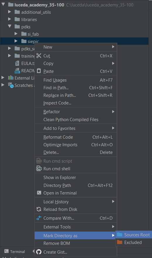
Mark the ipkiss folder of the Luceda PDK for SiEPIC as ‘Sources Root’
Now you can start using the Luceda PDK for SiEPIC in your designs.
2.2. Define the layout of the unit cell (+ create a new building block)
As explained previously, the unit cell is the basic building block of the WBG and will determine the properties of the whole device. To define it, we first need to tell IPKISS what the unit cell looks like.
Just like for the layout of the MMI in the MMI layout tutorial, we define a PCell for the unit cell that defines its full geometry.
We create a Python file cell.py in the grating_unit_cell folder in which we will store the unit cell and its layout:
class UnitCellRectangular(i3.PCell):
    """Unit cell of the WBG. It contains a wide center section with length L2 and width w2.
    It is surrounded by 2 waveguides with a width of w1 and combined length of L1.
    """

    _name_prefix = "uc_rect"
    trace_template = i3.TraceTemplateProperty(doc="Trace template of the unit cell waveguide sections")
    length1 = i3.PositiveNumberProperty(default=0.175, doc="Length of the narrow waveguide section")
    length2 = i3.PositiveNumberProperty(default=0.175, doc="Length of the wide waveguide section")
    width = i3.PositiveNumberProperty(default=0.5, doc="Average width of the grating")
    deltawidth = i3.PositiveNumberProperty(default=0.052, doc="Corrugation width")

    uc_attributes = ["length1", "length2", "width", "deltawidth"]

    def _default_trace_template(self):
        return pdk.WaveguideBraggGratingTemplate()

    class Layout(i3.LayoutView):
        def generate(self, layout):
            core_layer = self.trace_template.core_layer
            lambda_b = self.length1 + self.length2
            # Si core
            layout += i3.Rectangle(
                layer=core_layer,
                center=(0.25 * self.length1, 0.0),
                box_size=(0.5 * self.length1, self.width - self.deltawidth),
            )
            layout += i3.Rectangle(
                layer=core_layer,
                center=(0.5 * lambda_b, 0.0),
                box_size=(self.length2, self.width + self.deltawidth),
            )
            layout += i3.Rectangle(
                layer=core_layer,
                center=(0.75 * self.length1 + self.length2, 0.0),
                box_size=(0.5 * self.length1, self.width - self.deltawidth),
            )

            layout += i3.OpticalPort(
                name="in",
                position=(0.0, 0.0),
                angle=180.0,
                trace_template=pdk.StripWaveguideTemplate(),
            )
            layout += i3.OpticalPort(
                name="out",
                position=(lambda_b, 0.0),
                angle=0.0,
                trace_template=pdk.StripWaveguideTemplate(),
            )
            return layout
Since we focus on designing a rectangular unit cell, we name the class UnitCellRectangular. You can now see the following properties:
_name_prefix: prefix to the unit cell name. Since we have a rectangular unit cell, we set this property asuc_rect.trace_template: this property describes, among others, the cross section of the waveguides. Although SiEPIC offers only one cross section in which the silicon is fully etched (as compared to the generic SiFab that also offers shallowly etched waveguides), it does offer some freedom in regards to the resolution in which the structures are defined in the mask during the foundry’s postprocessing. Put shortly, a higher resolution will result in a lower amount of quantization errors on the final mask but will also result in a more costly and time consuming fabrication process. To alleviate the cost and time issues while still retaining sufficient resolution, shot pitch fracturing can be applied to the layout of WBGs. More information about shot pitch fracturing can be found here. To ensure shot pitch fracturing is applied to the unit cells (and thus WBGs), we set the trace template topdk.WaveguideBraggGratingTemplate(), contrary topdk.StripWaveguideTemplate()which is used for the routing waveguides and is drawn in a coarser resolution without shot pitch fracturing.The lengths
length1,length2, the average widthwidthand the corrugation widthdeltawidth: these properties fully describe the layout of the unit cell as illustrated in Layout parameters.
We also give UnitCellRectangular the property uc_attributes.
As explained in the previous section, the coefficients describing the optical properties of the unit cells will be stored in .txt files.
The name of the .txt file should hence reflect the layout of its corresponding unit cell.
For a rectangular unit cell, we have 5 properties: the shape of the unit cell (in our case rectangular) and the properties describing its layout: length1, length2, width and deltawidth.
The shape of the unit cell is already given by _name_prefix, so we need a list that contains the attributes describing the unit cell layout.
That list is the property uc_attributes.
Using both _name_prefix and uc_attributes, we will name the .txt file containing the polynomial fitting coefficients.

Layout parameters of a general rectangular unit cell: \(l_1\) (length1), \(l_2\) (length2), \(w\), (width) and \(\Delta w\) (deltawidth).
After the unit cell properties, we have the Layout class in which we define the shape of the unit cell based on the given properties.
As you can see, we define three rectangles corresponding to the shape of the rectangular unit cell.
More information about how to define the layout of a PCell can be found in the MMI layout tutorial.
The same applies to the port definition, which is done as part of the method generate(self, layout).
Note
Before you can import and use the unit cell PCell in an external script, you will need to add the folder luceda-academy/libraries/pteam_library_siepic/ipkiss to the PYTHONPATH.
This is done by marking this directory as ‘Sources Root’, as done for the SiEPIC PDK in Adding source folders.
The unit cell can now be instantiated with the Python file example_unit_cell.py found in the luceda-academy/training/topical_training/wbg_temp_sensor folder.
At the top of the file, we import the unit cell building block and other relevant packages.
We then define and visualise a unit cell with dimensions \(l_{1}=158\,\mathrm{nm}\), \(l_{2}=158\,\mathrm{nm}\), \(w=500\,\mathrm{nm}\) and \(\Delta w=50\,\mathrm{nm}\) using the following code:
uc = UnitCellRectangular(
    width=0.5,
    deltawidth=0.05,
    length1=0.158,
    length2=0.158,
)
uc_layout = uc.Layout()
uc_layout.visualize(annotate=True)
which is plotted in Unit cell layout:
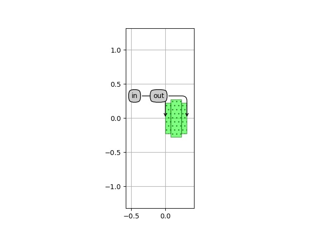
Unit cell layout
2.3. Calculating the S-parameters of the unit cell with CAMFR
Everything is now set for CAMFR to calculate the unit cell response, i.e. the S-matrices for different wavelengths and temperatures.
Unlike the MMI in the MMI simulation and optimization tutorial, the simulation recipe here is defined outside of the SiEPIC PDK, i.e. in the Luceda Academy tutorial, as the temperature dependence of the materials is not covered by the SiEPIC PDK.
Nevertheless, the simulation recipe still needs the information of the layer stacks as defined in the SiEPIC PDK.
Indeed, CAMFR turns the 3D layer stack of the SiEPIC foundry into a 2D grid of effective indices, and will then apply its EME methods to simulate the circuit.
The function that contains the CAMFR simulation recipe for the unit cell is called simulate_uc_by_camfr.
We assume there is no polarization conversion, meaning TE-polarized light coupling to TM-polarized modes and vice versa.
This will enable us to simulate the optical behaviour of the unit cell for TE and TM polarized light separately, which will save simulation time if our WBG only operates at one particular wavelength.
The simulation recipe simulate_uc_by_camfr takes the following parameters as input:
uc_object: the unit cell object, containing its attributes and Layout View, that you wish to simulate.wavelengths: a set of wavelengths to use for the simulation (ndarray, unless single value).temperatures: a set of temperatures to use for the simulation (ndarray, unless single value).discretization_res: the discretization resolution (default is 20), with the factor 1/discretisation_res defining what is the minimal change between the widths and lengths of consecutive slabs of a longitudinally variant structure.num_mod: the number of modes to simulate (default is 25).polarization: the polarization (string) of the light (default is ‘TE’).
and will output the following parameters (in this order):
sim_result[0]: the wavelengths for which the simulation is performed.sim_result[1]: the temperatures for which the simulation is performed.sim_result[2]: S-matrix coefficients describing the optical response of the unit cell for the given polarization, wavelengths and temperatures.
For our unit cell, which has two ports and is simulated at one particular polarization, there are four S-matrix coefficients:
\(T_{12}\): the transmission from the input port to the output port.
\(T_{21}\): the transmission from the output port to the input port.
\(R_{12}\): the reflection from the input port.
\(R_{21}\): the reflection from the output port.
These four S-matrix coefficients are thus calculated for a set of wavelengths and temperatures by the simulation recipe simulate_uc_by_camfr.
Since we are dealing with a multidimensional array of data for each of the four S-matrix coefficients (a set of wavelengths and a set of temperatures), handling and saving the dataset can be challenging.
To deal with these multidimensional datasets, simulate_uc_by_camfr outputs the simulation data for each S-matrix coefficient as a long array containing the results from both the wavelength and temperature sweeps.
This is illustrated in Storing 2D data as an array for \(T_{12}\), simulated for \(M_w\) wavelengths and \(M_t\) temperatures.
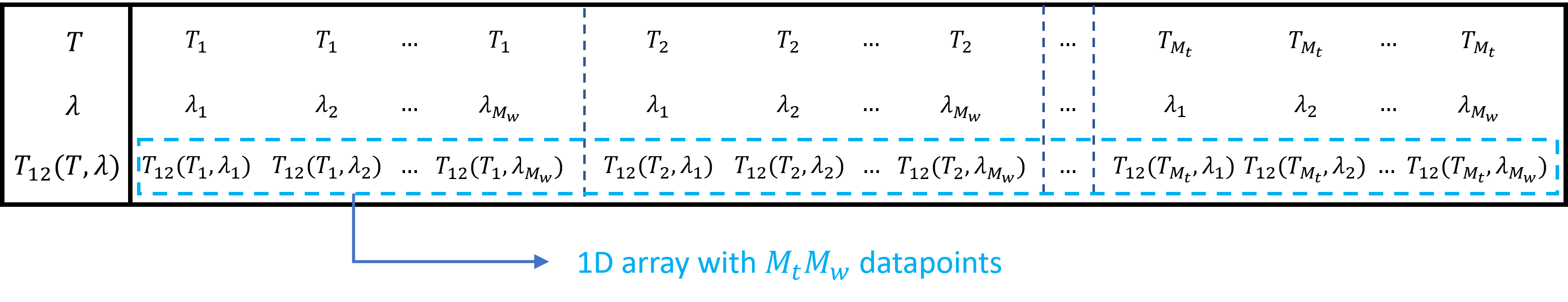
Illustration of how to store 2D data (\(T_{12}\) as a function of wavelength \(\lambda\) and temperature \(T\)) as a 1D array
More generally, multidimensional data of the form \(M_1\times M_2\times...\times M_n\) can be stored into a 1D array of length \(M_1M_2...M_n\) and retrieved if the dimensions \(M_1\times M_2\times...\times M_n\) are known as well.
So, for sim_result[2], the data is saved in a \(4\times M_wM_t\) matrix, with the first, second, third and fourth row corresponding to \(T_{12}\), \(T_{21}\), \(R_{12}\) and \(R_{21}\) respectively.
We now calculate, for TE-polarization, the unit cell S-matrix coefficients for wavelengths between 1400 nm to 1700 nm and at the temperatures \(T=273\,\mathrm{K}\) and \(T=300\,\mathrm{K}\).
In example_unit_cell.py, where we defined the unit cell PCell, we simply initiate simulate_uc_by_camfr with the following code:
print("Calculating the properties of the unit cell for different wavelengths and temperatures...")
sim_result = simulate_uc_by_camfr(
    uc_object=uc,
    wavelengths=np.arange(1.4, 1.7, 0.01),
    temperatures=np.array([273.0, 300.0]),
    num_modes=50,
    polarization="TE",
)
plot_smatrix_coefficients(sim_result)
with uc the unit cell PCell we initiated earlier, and where we take the sufficiently large number of modes of 50.
The S-matrix coefficients can then be plotted using the function plot_smatrix_coefficients and are depicted in S-matrix coefficients.
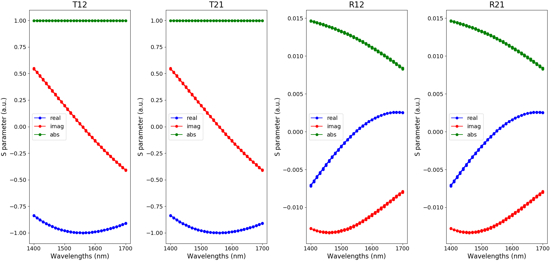
Illustration of the S-matrix coefficients as a function of wavelength and for the temperatures 273 K and 300 K (blue: real part, red: imaginary part and green: absolute value)
2.4. Fit and save the S-matrix coefficients to a .txt file
Now that we have calculated the S-matrix coefficients, we need to fit them with polynomials and save them in a text file. This data will be used for the circuit model of the unit cell and the WBG later on. Since we will place the WBG in a circuit using building blocks provided by the SiEPIC PDK, we need to ensure compatibility with the models from those building blocks. One key feature of the SiEPIC PDK components is that they take into account the optical performance for both the TE and TM polarizations. So, for our unit cell, we need to retrieve the component’s behavior at both the TE and TM polarizations as well.
To create and save the data necessary for the circuit models, we simply initiate the function create_uc_model_data() on the unit cell PCell uc in example_unit_cell.py:
create_uc_model_data(uc_pcell=uc)
which takes the following parameters:
uc_pcell: the unit cell PCell, containing its attributes and Layout View you wish to simulate.wavelengths: the set of wavelengths used for model fitting (default isnp.linspace(1.4, 1.7, 11)).temperatures: the set of temperatures used for model fitting (default isnp.linspace(173., 473., 7)).npoly_wavelengths: the order of the polynomial fitting for the wavelength dependence (default is 7).npoly_temperatures: the order of the polynomial fitting for the temperature dependence (default is 2).center_wavelength: the center wavelength around which the wavelength fitting occurs (default is 1.55).center_temperature: the center temperature around which the temperature fitting occurs (default is 273).plot_fitting: whether or not to plot the fitting to the S-matrix coefficients (default is False).
Most of the default values of these parameters are applicable for this WBG temperature sensor so we can simply pass on the unit cell object to create_uc_model_data().
Now, let’s take a look at the code in create_uc_model_data in more detail:
def create_uc_model_data(
    uc_pcell,
    wavelengths=np.linspace(1.4, 1.7, 11),
    temperatures=np.linspace(173.0, 473.0, 7),
    npoly_wavelengths=7,
    npoly_temperatures=2,
    center_wavelength=1.55,
    center_temperature=273.0,
    plot_fitting=False,
):
    print("Calculate the performance of the unit cell for different wavelengths and temperatures for TE polarisation.")
    uc_for_model_te = simulate_uc_by_camfr(
        uc_object=uc_pcell,
        wavelengths=wavelengths,
        temperatures=temperatures,
        num_modes=50,
        polarization="TE",
    )

    print("Calculate the performance of the unit cell for different wavelengths and temperatures for TM polarisation.")
    uc_for_model_tm = simulate_uc_by_camfr(
        uc_object=uc_pcell,
        wavelengths=wavelengths,
        temperatures=temperatures,
        num_modes=50,
        polarization="TM",
    )

    print("Retrieving the fitting coefficients.")
    te_fit_coeff = fit_camfr_data(
        sim_data=uc_for_model_te,
        npoly_wavelengths=npoly_wavelengths,
        npoly_temperatures=npoly_temperatures,
        center_wavelength=center_wavelength,
        center_temperature=center_temperature,
        plot_fitting=plot_fitting,
    )
    tm_fit_coeff = fit_camfr_data(
        sim_data=uc_for_model_tm,
        npoly_wavelengths=npoly_wavelengths,
        npoly_temperatures=npoly_temperatures,
        center_wavelength=center_wavelength,
        center_temperature=center_temperature,
        plot_fitting=plot_fitting,
    )

    print("Saving the fitting coefficients to a text file.")
    save_to_txt_files(uc_pcell, te_fit_coeff, tm_fit_coeff)
We can see that we perform two CAMFR simulations: one for TE-polarized light and one for TM-polarized light for which the simulation data is outputted in the variables uc_for_model_te and uc_for_model_tm respectively.
This data will then be fitted to a set of polynomials using the function fit_camfr_data.
Since we are dealing with multidimensional data here, fit_camfr_data will first do a polynomial fitting of the data around the center wavelength \(\lambda_0\) at each of the temperatures considered in the simulation data.
In other words, the polynomial fit of the S-parameters (along wavelength) has fitting coefficients that are dependent on the temperature.
For npoly_wavelengths equal to \(P_w\), this can be mathematically described as:
All the fitting coefficients \(p_i(T)\) for \(i=0,...,m\) are thus themselves functions - now dependent on the temperature - that can be fitted with a polynomial along \(T\) around the center temperature \(T_0\).
For npoly_temperatures equal to \(P_t\), each of the S-parameters will therefore be approximated by:
fit_camfr_data outputs the fitting coefficients \(p_{ij}\) in the te_fit_coeff and tm_fit_coeff matrices for TE- and TM-polarized light respectively.
It should be noted that the \(p_{ij}\) coefficients are stored in te_fit_coeff and tm_fit_coeff as \(8\times P_wP_t\) matrices, which is illustrated in Storing fitting coefficients.
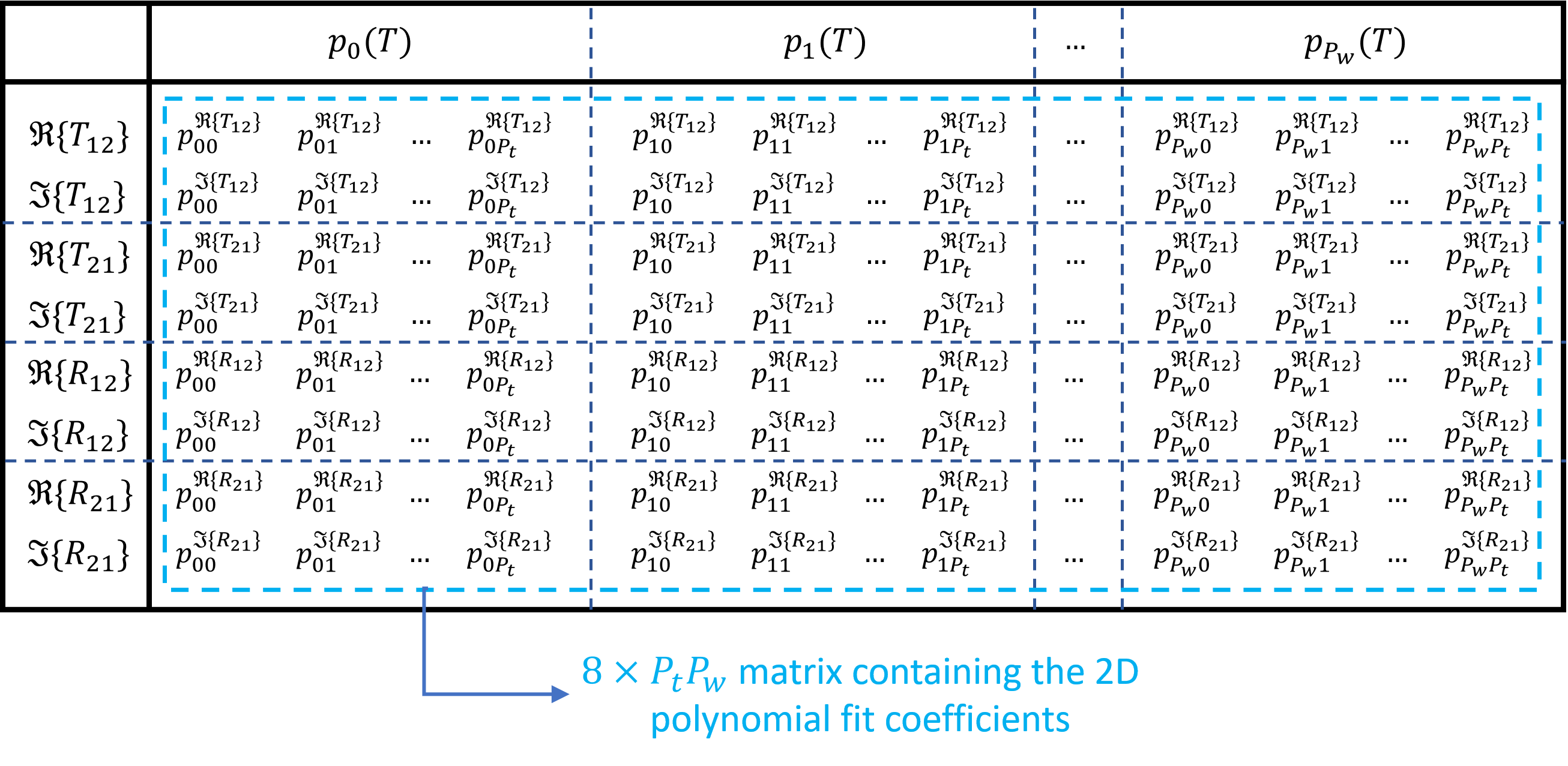
Illustration of how the \(p_{ij}\) fitting coefficients are stored for the four S-parameters for a given polarization (te_fit_coeff for TE and tm_fit_coeff for TM)
We need eight rows for the four S-parameters.
This is because we fit their real and imaginary parts separately as the fitting routines in NumPy can only deal with real numbers.
Finally, for both the te_fit_coeff and tm_fit_coeff matrices, the order of the polynomial fits and the center wavelength/temperature are saved to a .txt file using the function save_to_txt_files.
The .txt files will be saved in the folder model_data.
When looking at the name of the .txt file, you will see that it contains the shape of the unit cell configuration and its dimensions.
The folder also contains a file with the suffix ‘whats_there’ which includes the unit cell configurations for which there is simulation data.
To check whether the fitting does not yield unphysical behavior, we can plot the fitted data either directly with create_uc_model_data() by setting plot_fitting=True in example_unit_cell.py:
create_uc_model_data(uc_pcell=uc, plot_fitting=True)
This is illustrated here for TE in Fitted S-matrix coefficients:
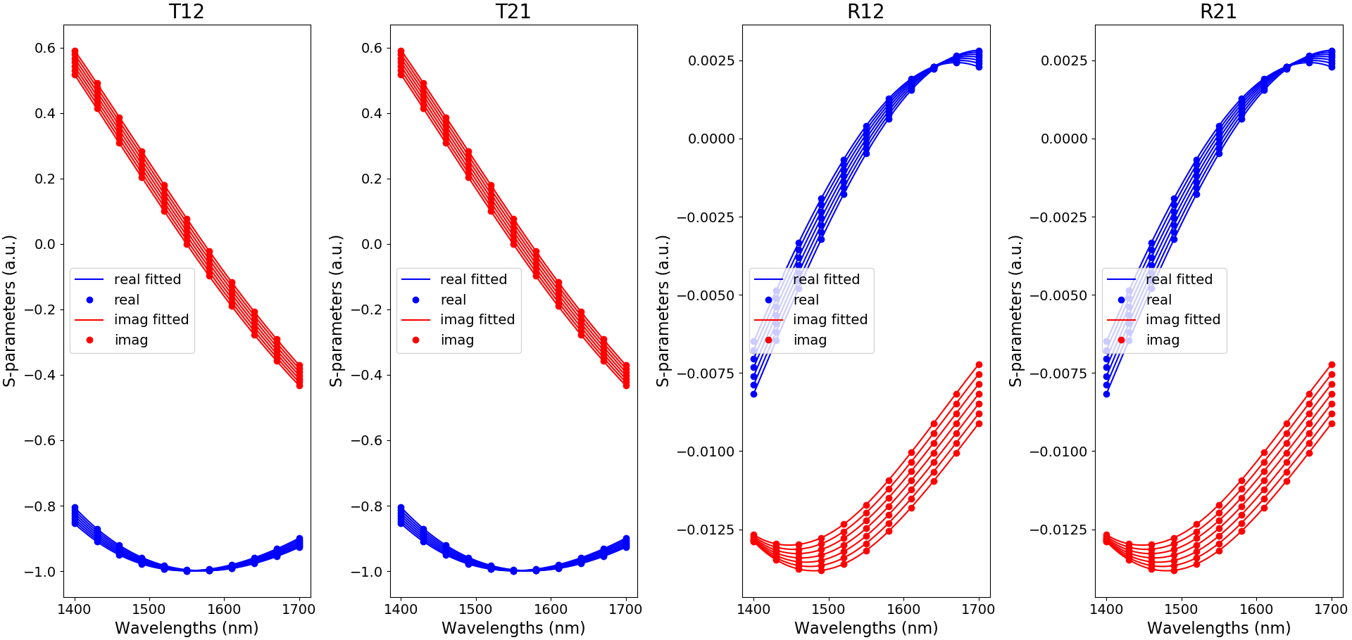
Fitted S-matrix coefficients for TE-polarization, as a function of wavelength and for the default temperatures used in create_uc_model_data (blue: real part and red: imaginary part)
or afterwards by invoking the show_model() function, which has the following parameters:
uc_pcell: the unit cell PCell which you want to visualise the model.wavelengths: the set of wavelengths at which you want to verify the model (np.array).temperatures: the set of temperatures at which you want to verify the model (np.array).
The results for the model of our unit cell are plotted in Fitted S-matrix coefficients TE/TM.
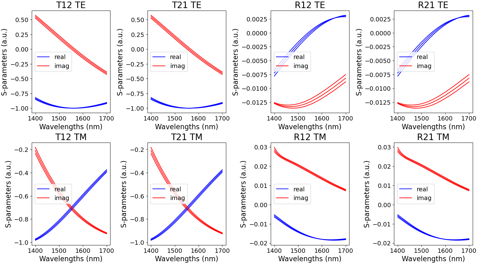
Fitted S-matrix coefficients for TE- and TM-polarization, as a function of wavelength and for the temperatures 200 K, 300 K and 400 K (blue: real part and red: imaginary part)
2.5. Define the circuit model of the unit cell
Now that we know how to generate and save the model data, we need to actually implement the circuit model in the unit cell component. We first create the netlist from the layout and ensure that each port contains two modes (TE and TM). To do so, we add the following code to the unit cell PCell:
class Netlist(pdk.NetlistFromLayout2Modes):
    pass
Implementing the circuit model itself, however, is done by including the CircuitModel class in the unit cell PCell:
    class CircuitModel(i3.CircuitModelView):
        def _generate_model(self):
            dims_smat_coeff, center_data, s_params_array = get_sparameters(uc_config=self.cell)
            return UnitCellModel(
                dims_smat_coeff=dims_smat_coeff, center_data=center_data, s_params_array=s_params_array
            )
Note that the temperature is not a parameter model, it will be taken from the environment later.
To retrieve the fitting data for the circuit model, we use the get_sparameters() function which takes just one parameter:
uc_config: the Pcell of the unit cell, from which we read the necessary attributes - since we invokeget_sparameters()within the unit cell PCell, this parameter is set atself.cell.
You can see we invoke it within the _generate_model method as it outputs the necessary information for the unit cell model in the following variables:
dims_smat_coeff: the dimensions of the matrix of fitting coefficients.center_data: center wavelength and temperature around which we fit.s_params_array: the array of fitting coefficients
get_sparameters() will also be used for the WBG as we will see later on.
The circuit model is then invoked with UnitCellModel() in _generate_model(self).
It has three parameters, dims_smat_coeff, center_data and s_params_array which are derived from the circuit model attributes as explained above.
The code for UnitCellModel() is given here:
class UnitCellModel(i3.CompactModel):
    parameters = [
        "dims_smat_coeff",
        "center_data",
        "s_params_array",
    ]
    terms = [i3.OpticalTerm(name="in", n_modes=2), i3.OpticalTerm(name="out", n_modes=2)]

    def calculate_smatrix(parameters, env, S):
        center_data, sdata_coeff = fit_sparameters(
            parameters.dims_smat_coeff, parameters.center_data, parameters.s_params_array, env.temperature
        )
        center_wavelength = center_data[0]
        sparam_fitted = [
            np.polyval(
                sdata_coeff[2 * index, :],
                env.wavelength - center_wavelength,
            )
            + 1j
            * np.polyval(
                sdata_coeff[2 * index + 1, :],
                env.wavelength - center_wavelength,
            )
            for index in range(8)
        ]

        S["in:0", "out:0"] = sparam_fitted[0]
        S["out:0", "in:0"] = sparam_fitted[1]
        S["in:0", "in:0"] = sparam_fitted[2]
        S["out:0", "out:0"] = sparam_fitted[3]
        S["in:1", "out:1"] = sparam_fitted[4]
        S["out:1", "in:1"] = sparam_fitted[5]
        S["in:1", "in:1"] = sparam_fitted[6]
        S["out:1", "out:1"] = sparam_fitted[7]
As you can see, the number of modes n_modes in i3.OpticalTerm is 2.
This is because we take into account both the TE and TM behavior of the unit cell in our models.
At the beginning of S-matrix calculation, we call fit_sparameters() with the arguments we obtained from get_sparameters() and with the temperature that we read from the env variable, just like the wavelength. fit_sparameters() will also be used in the same way for the WBG S-matrix. It outputs the following:
center_data[0]: the center wavelength for which the wavelength polynomial coefficients are retrieved.center_data[1]: the center temperature for which the temperature polynomial coefficients are retrieved. It is not used here, but can be useful for debugging.sdata_coeff: the wavelength polynomial coefficients for the S-parameters at the given temperature.
Furthermore, we see that polynomial fitting is done using Horner’s method.
Finally, we see that the port names in the S-parameter library take an integer as a suffix such that the entries are accessed by, for example, S['in:0', 'out:0'] or S['in:1', 'out:1'].
Again, this is due to the fact we have both TE and TM behavior taken into account in our model; 0 corresponds to the TE-modes while 1 indicates TM-polarized light.
Now that the unit cell model has been implemented in its PCell, we can initiate it and plot it as follows in example_unit_cell.py (taking a temperature of 300 K as an example):
wavelengths = np.linspace(1.5, 1.6, 2501)
uc_cm = uc.CircuitModel()
S = uc_cm.get_smatrix(wavelengths=wavelengths, temperature=300.0)
S.visualize(term_pairs=[("in:0", "out:0"), ("in:0", "in:0"), ("in:1", "in:1"), ("in:1", "out:1")])
As an illustration, we plot the reflection at the input port and the transmission from the input to the output port for both TE- and TM-polarized light in Transmission and reflection spectra.
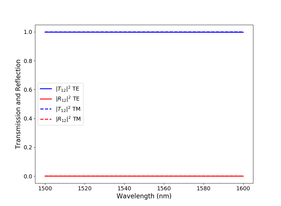
Absolute value of the S-matrix coefficients calculated at a temperature of 300 K over a wavelength range of 100 nm around 1550 nm with the generated unit cell model.
While this result might not mean much yet, we can now finally start optimizing the unit cell (and thus the WBG) configuration for temperature sensing and use its circuit model when characterizing the final circuit.