4. Creating the WBG layout and circuit model
In the previous section, we showed how to optimize the unit cell configuration in order to achieve the highest possible temperature sensitivity. Now, we need to stitch a number of these unit cells together in order to create the waveguide Bragg grating (WBG) used for temperature sensing, as we assume the WBG to be uniform (i.e. the unit cell configuration is constant over the whole WBG). To do so, we need to know how to
create the layout for the WBG, and
create the circuit model for the WBG.
4.1. Creating the WBG layout
The generation of the uniform WBG layout from the unit cell is fairly straightforward and is shown in the code below.
class UniformWBG(i3.PCell):
    _name_prefix = "uniform_wbg"
    uc = i3.PCellProperty(doc="Unit cell of the WBG.")
    n_uc = i3.IntProperty(default=25, doc="Number of unit cells in the WBG.")

    def _default_uc(self):
        return UnitCellRectangular(name=self.name + "_uc")

    class Layout(i3.LayoutView):
        def generate(self, layout):
            uc_layout = self.uc.get_default_view(i3.LayoutView)
            lambda_b = uc_layout.size_info().get_width()
            layout += i3.ARefX(
                self.uc,
                origin=(0, 0),
                n_o_periods_1d=self.n_uc,
                period_1d=lambda_b,
                name="uc",
            )

            wbg_aref = layout["uc"]
            layout += wbg_aref.ports[0]  # first port of the first period
            layout += wbg_aref.ports[-1]  # last port of the last period
            return layout
The properties we need are:
_name_prefix: the prefix of the WBG component’s name.uc: the unit cell PCell.n_uc: the number of unit cells.
The uniform WBG consists of n_uc references to uc stitched together.
To save on memory and processing speed, we create only one uc object and instantiate an array of references to it using ‘i3.ARefX’.
This array will be the only instance of our PCell, rather than having multiple instances for each individual unit cell.
Furthermore, from the unit cell uc and from the positions of the first and last references to it, we calculate the positions of the ports of the full WBG.
We are now ready to generate the final WBG. First, we create the object for the optimized unit cell. Then, we initiate a WBG based on 200 of these unit cells. The example code is given here:
width = 0.5
deltawidth = 0.088
dc = 0.2
lambdab = 0.325

uc = UnitCellRectangular(
    width=width,
    deltawidth=deltawidth,
    length1=(1 - dc) * lambdab,
    length2=dc * lambdab,
)
wbg = UniformWBG(uc=uc, n_uc=200)
wbg_lo = wbg.Layout()
wbg_lo.visualize(annotate=True)
Part of the WBG layout is depicted in Part of WBG.
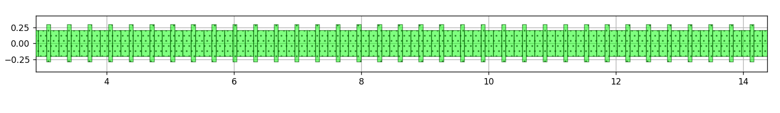
Zoomed into a part of the 300 period long WBG.
4.2. Creating the WBG circuit model
The circuit model for the WBG can now be generated in two ways:
From CAPHE simulations: the WBG is treated as a circuit. First, the S-matrix of each unit cell is calculated. Then, the resulting S-matrices are multiplied with each other to obtain the final S-matrix of the WBG.
Implement the model analytically by calculating the S-matrix of the unit cell and multiplying the matrices with each other.
In this section, we will focus on the second strategy.
The first strategy requires the S-parameters to be calculated n_uc times, but since we are dealing with a uniform grating, we only need to calculate the S-parameters once and then multiply the S-matrices accordingly.
This is a different approach from using CAPHE and will treat the WBG in the circuit model as one single building block rather than a cascade of n_uc unit cells.
Nevertheless, as we will see at the end of this section, when dealing with non-uniform gratings in which the unit cell configuration changes along the WBG, the CAPHE-based simulation is the preferred method due to straightforward implementation.
The availability of a variety of approaches demonstrates the versatility and flexibility of IPKISS when designing your components for a specific application.
To implement the WBG circuit model directly, we include the following class inside the WBG PCell:
    class CircuitModel(i3.CircuitModelView):
        def _generate_model(self):
            dims_smat_coeff, center_data, s_params_array = get_sparameters(self.uc)
            return UniformWBGModel(
                n_uc=self.n_uc,
                dims_smat_coeff=dims_smat_coeff,
                center_data=center_data,
                s_params_array=s_params_array,
            )
We can see that the code is almost identical to the code for the unit cell circuit model, with the main difference being that the circuit model is invoked with UniformWBGModel() in _generate_model(self) instead of UnitCellModel() because we now have an extra parameter, namely the number of unit cells n_uc.
The code for the WBG circuit model now is given in UniformWBGModel:
class UniformWBGModel(i3.CompactModel):
    _model_type = "python"
    parameters = [
        "n_uc",
        "dims_smat_coeff",
        "center_data",
        "s_params_array",
    ]
    terms = [i3.OpticalTerm(name="in", n_modes=2), i3.OpticalTerm(name="out", n_modes=2)]

    def calculate_smatrix(parameters, env, S):
        center_data, sdata_coeff = fit_sparameters(
            parameters.dims_smat_coeff, parameters.center_data, parameters.s_params_array, env.temperature
        )
        center_wavelength = center_data[0]
        sparam_fitted = [
            np.polyval(
                sdata_coeff[2 * index, :],
                env.wavelength - center_wavelength,
            )
            + 1j
            * np.polyval(
                sdata_coeff[2 * index + 1, :],
                env.wavelength - center_wavelength,
            )
            for index in range(8)
        ]

        sbar_te = (1 / sparam_fitted[1]) * np.array(
            [
                [sparam_fitted[0] * sparam_fitted[1] - sparam_fitted[2] * sparam_fitted[3], sparam_fitted[3]],
                [-sparam_fitted[2], 1.0],
            ]
        )
        smat_te = np.linalg.matrix_power(sbar_te, parameters.n_uc)
        sbar_tm = (1 / sparam_fitted[5]) * np.array(
            [
                [sparam_fitted[4] * sparam_fitted[5] - sparam_fitted[6] * sparam_fitted[7], sparam_fitted[7]],
                [-sparam_fitted[6], 1.0],
            ]
        )
        smat_tm = np.linalg.matrix_power(sbar_tm, parameters.n_uc)

        S["in:0", "out:0"] = 1 / smat_te[1][1]
        S["in:0", "in:0"] = -smat_te[1][0] / smat_te[1][1]
        S["out:0", "out:0"] = smat_te[0][1] / smat_te[1][1]
        S["out:0", "in:0"] = smat_te[0][0] + (smat_te[1][0] * smat_te[0][1] / smat_te[1][1])
        S["in:1", "out:1"] = 1 / smat_tm[1][1]
        S["in:1", "in:1"] = -smat_tm[1][0] / smat_tm[1][1]
        S["out:1", "out:1"] = smat_tm[0][1] / smat_tm[1][1]
        S["out:1", "in:1"] = smat_tm[0][0] + (smat_tm[1][0] * smat_tm[0][1] / smat_tm[1][1])
We can see it is a bit more complex than the code for the unit cell in UnitCellModel.
This is because the S-parameters for the unit cell can simply be described with the polynomial fit at the desired wavelengths.
For the full WBG however, we not only need to interpolate the S-matrix coefficients at the desired wavelengths, but we also need to restructure the resulting S-matrix.
Indeed, the regular S-matrix connects the ingoing fields with the outgoing fields.
But to connect the fields at the input port of the unit cell with those at its output port (in both cases both in- and outgoing), which is necessary to easily calculate the S-matrix of the full WBG, we need to restructure the S-matrix as follows:
We then take the \(n_{uc}\)-th power of this restructured S-matrix \(\bar{S}\) to calculate the (restructured) S-matrix of the total WBG, \(\bar{S}^{tot}\).
From this matrix, we finally retrieve the S-parameters for the full WBG: \(T_{12}^{tot}\), \(T_{21}^{tot}\), \(R_{12}^{tot}\) and \(R_{21}^{tot}\). These calculations are performed for both TE- and TM-polarized light.
Now that the circuit model is implemented, we can simulate our WBG.
An example is shown in example_full_wbg.py, where the WBG is simulated at the temperature of 293 K:
wavelengths = np.linspace(1.4, 1.7, 10001)
wbg_cm = wbg.CircuitModel()
S = wbg_cm.get_smatrix(wavelengths=wavelengths, temperature=300.0)

# plot the reflection and transmission spectra
We plot the reflection and transmission spectra for TE and TM from \(1.4\,\mathrm{\mu m}\) to \(1.7\,\mathrm{\mu m}\) in Transmission spectra.
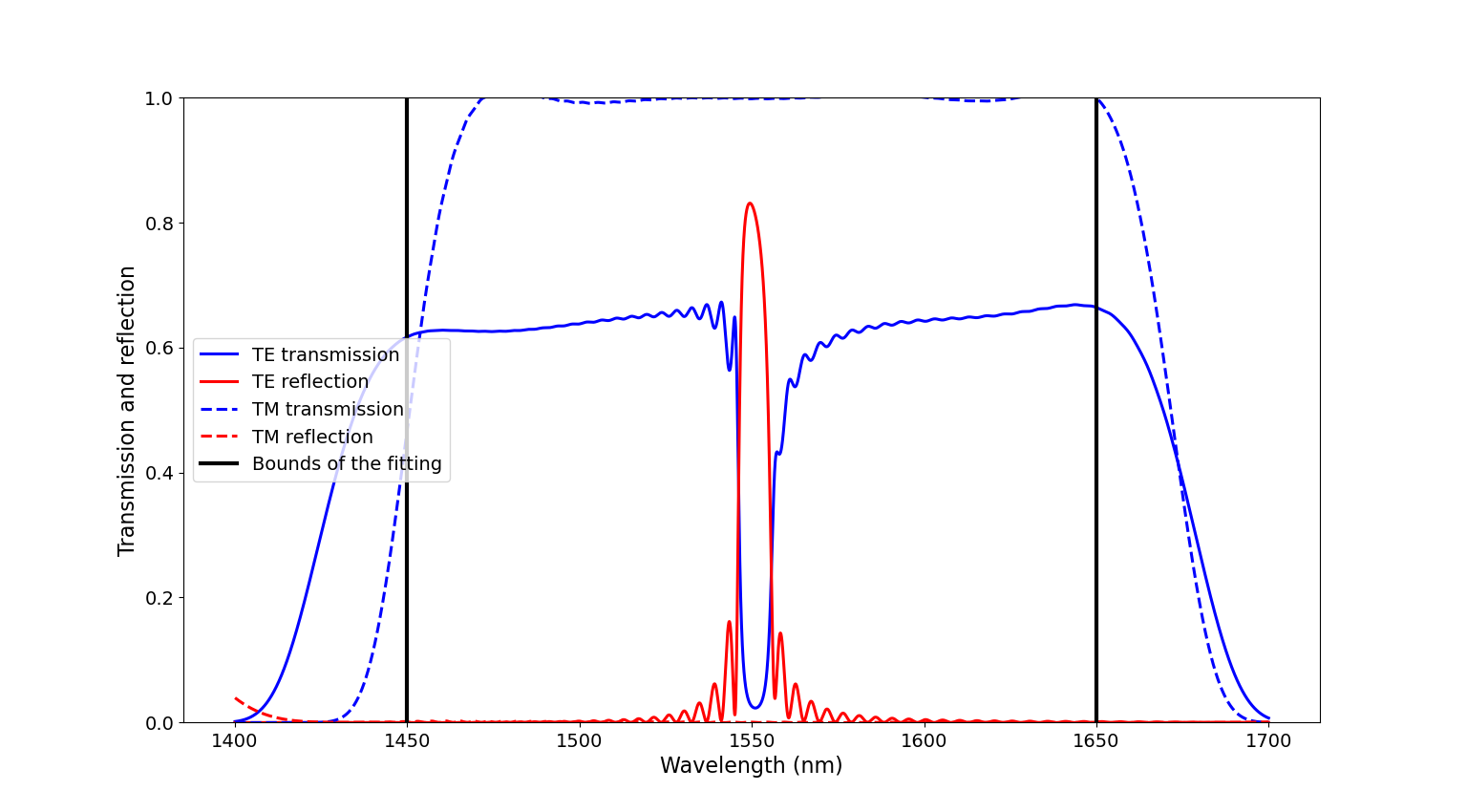
Transmission (blue) and reflection (red) spectra for TE (full line) and TM (dashed line) light at the operating temperature (293 K). The vertical black lines indicate the bounds of the wavelength range for which the model of the unit cell was determined and fitted.
A large reflection peak is clearly visible around 1550 nm for TE-polarized light, which is what we expected. No reflection peak is present for TM-polarized light, meaning that this particular WBG is not suited for TM-polarized operation. Another important feature to notice is that the model breaks down for wavelengths outside of the fitting range. It is therefore important to not characterize circuits outside of the wavelength range for which they are fitted, as unwanted artefacts can pop up.
To illustrate the temperature sensing operation of the WBG, we calculate the reflection at different temperatures within and outside the range in which our sensor operates. The code is given below:
wavelengths = np.linspace(1.45, 1.65, 10001)
temperatures = [193.0, 243.0, 293.0, 343.0, 393.0, 443.0]
lambdac_vals = []

for temperature in temperatures:
    S = wbg_cm.get_smatrix(wavelengths=wavelengths, temperature=temperature)
    reflection_te = i3.signal_power(S["in:0", "in:0"])
    lambdac_vals.append(wavelengths[np.where(reflection_te == np.max(reflection_te))[0][0]])
    plt.plot(wavelengths * 1000, reflection_te, "-", linewidth=2.2, label=r"T=" + str(temperature) + " K")

plt.xlabel(r"Wavelength (nm)", fontsize=16)
plt.ylabel("Reflection", fontsize=16)
plt.legend(fontsize=14, loc=6)
plt.ylim([0.0, 1.0])
plt.tick_params(which="both", labelsize=14)
plt.show()
The results are depicted in Reflection spectra:
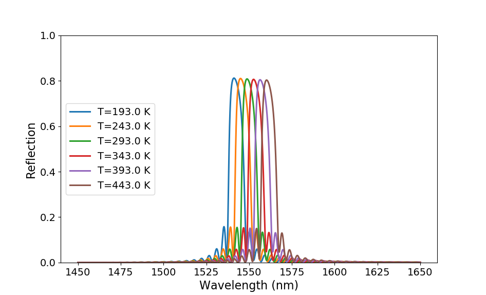
Reflection spectra for TE for different temperatures.
This plot clearly shows that an increase in temperature shifts the center of the reflection band at \(\lambda_c\) to longer wavelengths. When plotting \(\lambda_c\) as a function of temperature (Temperature Offset of the center wavelength), we can see that there is a linear relationship between the wavelength and the temperature. The plot also shows our sensor has the potential to properly operate beyond the range of temperatures for which it was originally designed.
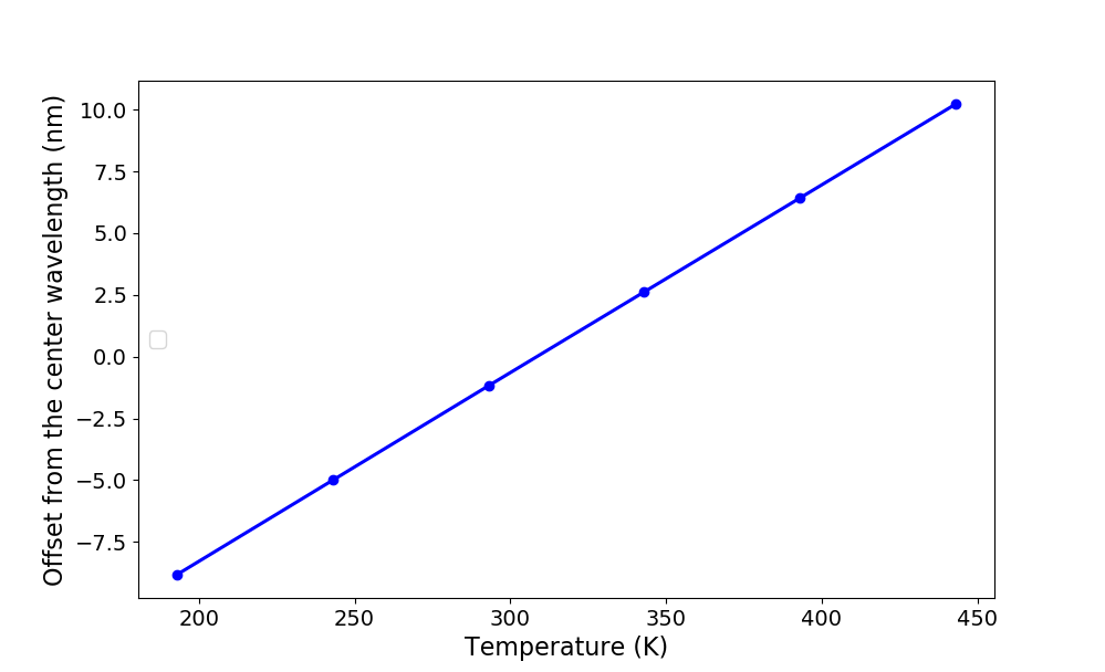
Offset of the WBG center wavelength \(\lambda_c\) from \(1.55\,\mathrm{\mu m}\) as a function of the temperature.
4.3. Test your knowledge
As explained in the previous section, instead of directly implementing the WBG circuit model, we can also rely on Caphe to generate the WBG circuit model from the set of unit cells automatically.
For a general grating, consisting of an arbitrary number of unit cells of arbitrary configuration, the S-matrix coefficients can be calculated with CAPHE by rewriting the CircuitModel class in the WBG PCell as:
class CircuitModel(i3.CircuitModelView):
    def _generate_model(self):
        return i3.HierarchicalModel.from_netlistview(self.netlist_view)
provided that the components (in this case the unit cells) are all stitched together properly. In other words, the input and output ports for each of the adjacent components need to overlap.
Although this increases the time to generate the circuit model, it provides much more freedom in regards to the types of WBG you want to simulate. An example of gratings that need to rely on the CAPHE-based circuit model implementation are apodized WBGs. In an apodized WBG, \(\Delta w\) gradually increases from the input port to its maximum value \(\Delta w_{max}\), typically in the center of the WBG, and then decreases again towards the output of the WBG. When the corrugation width follows a Gaussian profile [Ma2018], the corrugation width of the \(i\)-th unit cell in a WBG with \(n_{uc}\) unit cells can be calculated as:
with \(\alpha\) the apodization factor determining the ‘FWHM’ of the grating profile. Note that when \(\alpha=0\), you end up with a regular uniform grating. An illustration of such an apodized WBG is given in Apodized grating.
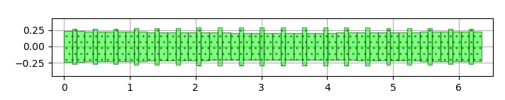
Illustration of an apodized grating.
We now ask you to design and model an apodized WBG with a rectangular unit cell that operates at a center wavelength of \(\lambda_c=1.54\,\mathrm{\mu m}\). We keep the average width \(w\) fixed at 500 nm and the duty cycle at 0.2, while \(\Delta w_{max}\) is taken as 88 nm. You should create both the layout and the circuit model of this apodized WBG. In order to help you finish this exercise, we list the necessary challenges you need to tackle:
The corrugation width \(\Delta w\) has an effect on the center wavelength \(\lambda_c\). This means that, not only the corrugation width changes along the WBG, but also the grating period \(\lambda_B\). Thus, the first thing to do is, for each value of \(\Delta w\), find the value of \(\lambda_B\) that yields a center wavelength of \(\lambda_c=1.54\,\mathrm{\mu m}\). We refer to the previous section, in which we searched for the unit cell configurations yielding a particular \(\lambda_c\), for inspiration.
Create an apodized WBG PCell, containing the Layout and CircuitModel classes. Regarding the CircuitModel class, keep in mind that for the circuit model to work, you need .txt files containing simulation data for each value of \((\Delta w,\Lambda_B)\) used in the WBG. Hence, you should create the .txt files for a set of \((\Delta w,\Lambda_B)\) configurations. These configurations will also be used to create the layout of the apodized WBG, whose corrugation width profile follows Eq. (1). Make sure that the parameter \(\alpha\) is an attribute of the apodized WBG’s PCell. We advise you to use steps of 2 nm in the range of \(\Delta w\) values.
Calculate the reflection spectra for both the apodized WBG and the uniform WBG.
The solution of the exercise is provided in execute_solution_test_your_knowledge.py and section04_solution_test_your_knowledge_pcell.py, the latter file containing the PCell of the apodized WBG.
When you run execute_solution_test_your_knowledge.py, it will plot three figures:
It will first show the \((\Delta w,\Lambda_B)\) configurations that yield a center wavelength of \(\lambda_c=1.54\,\mathrm{\mu m}\), shown in Parameter configurations.
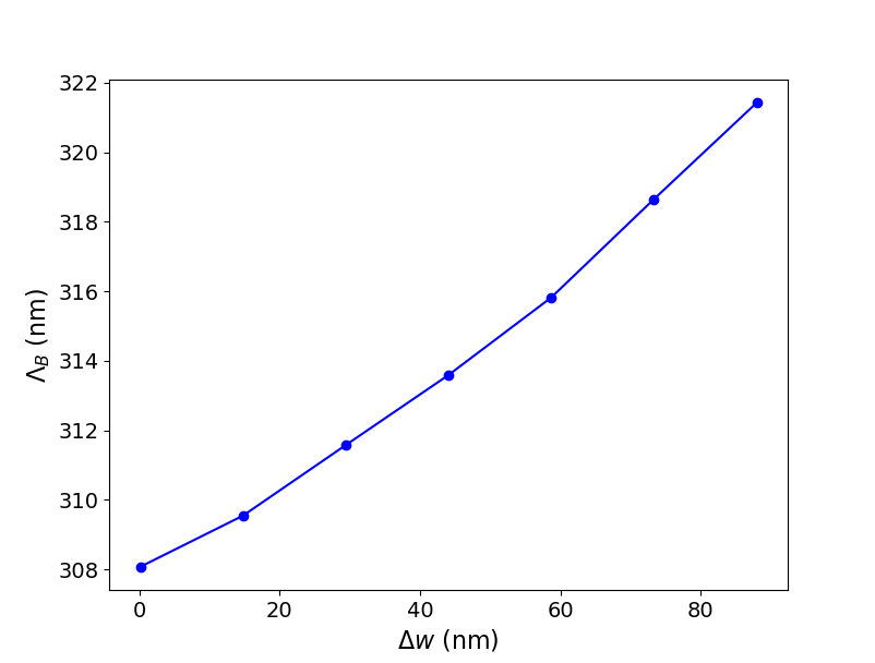
\((\Delta w,\Lambda_B)\) configurations that attain \(\lambda_c=1.54\,\mathrm{\mu m}\).
Then it will generate the .txt files containing the S-parameter data for a number of \((\Delta w,\Lambda_B)\) configurations (this can take a while). The apodized WBG is invoked for \(\alpha=4\) and for \(\alpha=0\), the latter yielding the uniform grating, as well as the uniform WBG as described earlier in this section with the custom circuit model. The reflection spectra is calculated for these WBGs and the results are plotted in Reflection spectrum simulations.
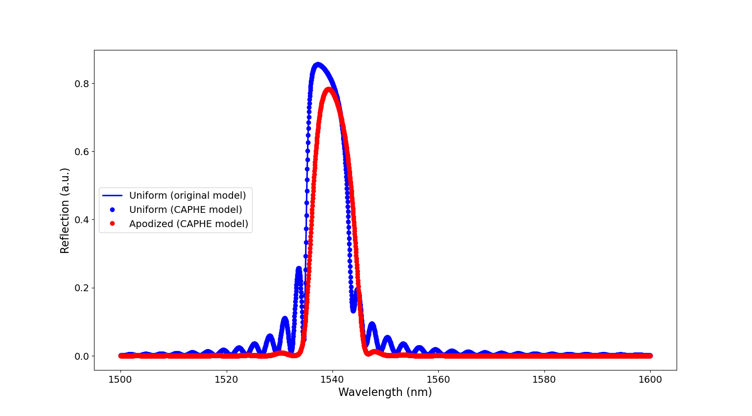
Reflection spectrum of the uniform grating calculated with the custom circuit model (full line) and CAPHE (blue circles) together with the reflection spectrum of the apodized WBG (red circles).
Finally, the script calculates the reflection spectra for different temperatures and plots the results in Reflection spectra apodized WBG.
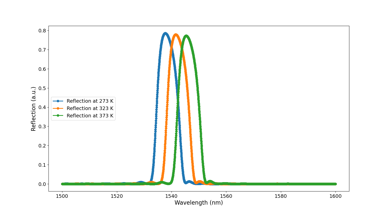
Reflection spectra of the apodized WBG for different temperatures.
We can see that apodizing the WBGs results in ‘cleaner’ reflection spectra, in which the side bands are greatly suppressed compared to the uniform WBGs. We also see that the reflection spectra for the uniform WBG are exactly the same between the one calculated with CAPHE and the one calculated with the custom circuit model described earlier in this section. This is therefore a nice validation of our custom circuit model for the uniform grating. It shows that it is reliable, with the added benefit of it being faster than WBG circuit model calculated with CAPHE.
For this reason, we will decide to continue with the uniform grating in creating the full sensor circuit in the next section.
Ma et al., “Apodized Spiral Bragg Grating Waveguides in Silicon-on-Insulator,” in IEEE Photonics Technology Letters, vol. 30, no. 1, pp. 111-114, 1 Jan.1, 2018, doi: 10.1109/LPT.2017.2777824