3. Optimizing the temperature sensitivity

In the previous section, we showed how to use IPKISS and, in particular, CAMFR to create the layout and to simulate the optical properties of a unit cell in the WBG. We also saw how these optical properties can be fitted with a set of polynomials and exported to a .txt file in order to generate the unit cell’s circuit model later on. In this section, we will use CAMFR to optimize the unit cell to achieve maximal temperature sensitivity. In particular, you will learn how to:

find the configurations that yield a center wavelength of \(\lambda_c\),
find the configuration yielding the most sensitive temperature sensing,
simulate the temperature sensing of the device and export the data for use in the circuit model.

3.1. Configurations at \(\lambda_c\)

We want our temperature sensor to operate at a center wavelength of \(\lambda_c=1.55\,\mathrm{\mu m}\) which means that the WBG should have a maximal reflection at this \(\lambda_c\). This means that we first have to calculate the layout parameters of the unit cell yielding this particular \(\lambda_c\). To lower the amount of optimization sweeps we need to perform, we keep the average width of the grating fixed at \(w=500\,\mathrm{nm}\) as this is the standard waveguide width in the SiEPIC platform. We will then vary the other three variables of the unit cell: the corrugation width \(\Delta w\) and the lengths \(l_1\), \(l_2\) by sweeping the Bragg period \(\Lambda_B\) and the duty cycle \(\mathcal{D}\) through \(l_1=(1-D)\Lambda_B\) and \(l_2=D\Lambda_B\). In our unit cell example, we will sweep \(\Delta w\) from 10 nm to 150 nm, \(\Lambda_B\) from 250 nm to 400 nm and \(\mathcal{D}\) from 0.2 to 0.8. More specifically, for each set of \(\left(\Lambda_B,\,\mathcal{D}\right)\), we will calculate the value of \(\Delta w\) for which we have a \(\lambda_c=1.55\,\mathrm{\mu m}\). This is done with the following code:

example_optimize_temperature_sensitivity.py

width = 0.5  # average width of the grating
lambdac = 1.55  # operating wavelength
tc = 293  # operating temperature
polarization = "TE"  # operating polarization


########################################################################################################################
# Define the variable sweeps. Then find the configurations that have a center wavelength of lambda_c.
########################################################################################################################

print(" ")
print("Finding the configurations that yield a center wavelength of {} um".format(lambdac))

deltawidth_values = np.linspace(0.01, 0.15, 15)
lambdab_values = np.linspace(0.25, 0.4, 13)
dc_values = np.linspace(0.2, 0.8, 7)

configurations = []
for lambdab in lambdab_values:
    for dc in dc_values:
        phase_values = []
        for deltawidth in deltawidth_values:
            uc = UnitCellRectangular(
                width=width,
                deltawidth=deltawidth,
                length1=(1 - dc) * lambdab,
                length2=dc * lambdab,
            )
            sim_result = simulate_uc_by_camfr(
                uc_object=uc,
                wavelengths=lambdac,
                temperatures=tc,
                num_modes=50,
                polarization=polarization,
            )
            Smat = sim_result[2]
            phase_uc = np.angle(Smat[0][0] * Smat[1][0]) / np.pi
            phase_values.append(phase_uc)

        deltawidth_interp = np.linspace(deltawidth_values[0], deltawidth_values[-1], len(deltawidth_values) * 1000)
        phase_values_interp = np.abs(
            interp1d(
                deltawidth_values,
                np.unwrap(np.array(phase_values)),
                kind="cubic",
            )(deltawidth_interp),
        )  # calculate the phase values on a finer deltawidth grid (on deltawidth_interp)
        min_index = np.where(phase_values_interp == np.min(phase_values_interp))
        if (min_index[0][0] != 0) and (min_index[0][0] != (deltawidth_interp.__len__() - 1)):
            deltawidth_c = deltawidth_interp[min_index[0][0]]
            configurations.append((lambdab, dc, deltawidth_c))

To find the center wavelength of the resulting WBG from a certain unit cell configuration, we have to look at the wavelength for which the reflections of two consecutive unit cells constructively interfere. Mathematically, this means that the roundtrip phase \(T_{12}T_{21}\) is an integer multiplication of \(2\pi\). As such, we look for the \(\Delta w\) values for which the condition \(T_{12}T_{21}=2\pi\) holds. If this value is within the range of \(\Delta w\), we save the set \(\left(\Delta w,\,\Lambda_B,\,\mathcal{D}\right)\) into an array configurations that will be used later for the temperature sensitivity optimization.

For the given values in \(\left(\Delta w,\,\Lambda_B,\,\mathcal{D}\right)\) space, the configurations that yield a center wavelength at \(\lambda_c=1.55\,\mathrm{\mu m}\) are plotted in Unit cell configurations (this can take a few minutes to simulate).

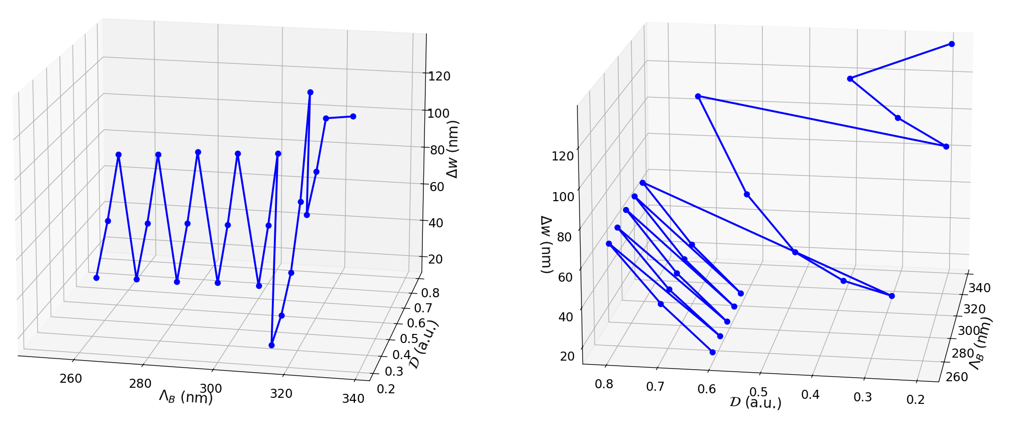
../../../_images/Configurations.png — Unit cell configurations that yield a center wavelength of \(\lambda_c=1.55\,\mathrm{\mu m}\)

3.2. Find the configuration yielding the most sensitive temperature sensor

Now that we have found all the unit cell configurations that work at the desired operating wavelength, we can find the one that yields the most sensitive temperature sensor. To do so, we have to look at which configuration yields the largest change in \(\lambda_c\) for a particular temperature change \(\Delta T\). Because the value of \(\lambda_c\) is strongly tied to the roundtrip phase, as explained before, we can simply look at the change in roundtrip phase as a result of the temperature variations, rather than calculating \(\lambda_c\) directly. For each of the stored unit cell configurations in configurations, we thus calculate the roundtrip phase change in case we have a temperature variation of \(\Delta T=2\,\mathrm{K}\). The code is given below:

example_optimize_temperature_sensitivity.py

phase_change = []
for config in configurations:
    uc = UnitCellRectangular(
        width=width,
        deltawidth=config[2],
        length1=(1 - config[1]) * config[0],
        length2=config[1] * config[0],
    )

    sim_result = simulate_uc_by_camfr(
        uc_object=uc,
        wavelengths=lambdac,
        temperatures=np.array([tc - 1, tc + 1]),
        num_modes=50,
        polarization=polarization,
    )
    Smat = sim_result[2]
    phase_uc_m = np.angle(Smat[0][0] * Smat[1][0]) / np.pi
    phase_uc_p = np.angle(Smat[0][1] * Smat[1][1]) / np.pi

    phase_for_delta = np.unwrap(np.array([phase_uc_m, phase_uc_p]))
    phase_change.append(abs(phase_for_delta[1] - phase_for_delta[0]))

best_index = np.where(phase_change == np.max(phase_change))
best_configuration = configurations[best_index[0][0]]

The calculated sensitivities (in rad/K) are given in Configuration sensitivity for each configuration that has a center frequency of \(\lambda_c\).

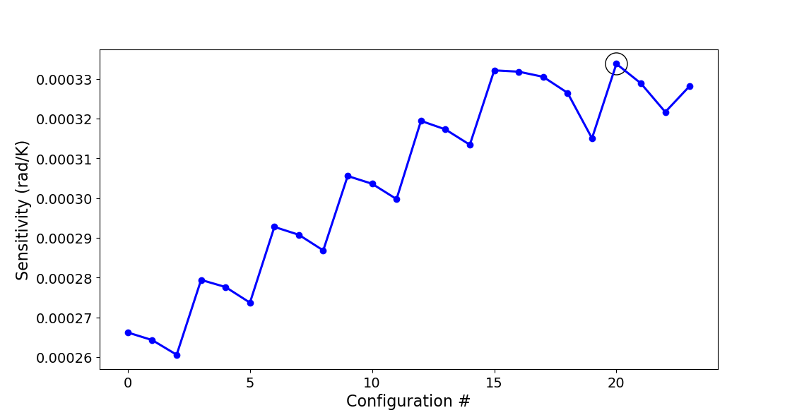
../../../_images/uc_sensitivities.png — Sensitivities (in rad/K) of all the configurations yielding a center wavelength of \(\lambda_c\). The most sensitive configuration is indicated with a black circle.

We find that the optimum unit cell has the following properties: \(\Delta w=89\,\mathrm{nm}\), \(\Lambda_B=325\,\mathrm{\mu m}\) and \(\mathcal{D}=0.2\). When creating the unit cell PCell, its layout can be generated and visualized with the following code:

uc = UnitCellRectangular(
    width=width,
    deltawidth=best_configuration[2],
    length1=(1 - best_configuration[1]) * best_configuration[0],
    length2=best_configuration[1] * best_configuration[0]
)
uc_layout = uc.Layout()
uc_layout.visualize(annotate=True)

and it is depicted in Optimized unit cell configuration.

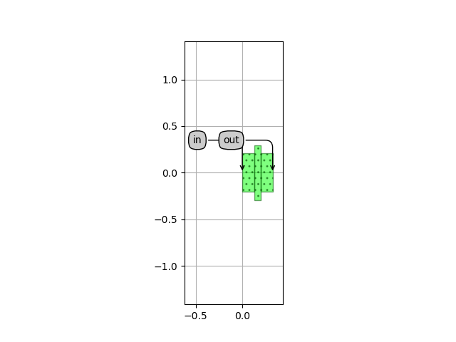
../../../_images/UC_mostsensitive.png — Optimized unit cell configuration yielding the best temperature sensitivity

3.3. Simulate the temperature sensing of the device

Now that we optimized the unit cell for highest temperature sensitivity, let’s take a look at the S-matrix coefficients for different temperatures. As we already have defined the optimized unit cell object, we can create its circuit model following the recipe outlined in the previous section. We will fit the model within the boundaries imposed by the application. In our case, we decide that the temperature sensor should operate between \(-25\,^\circ\mathrm{C}\) and \(125\,^\circ\mathrm{C}\), and that we should be able to measure the reflection spectra over a wavelength range of \(200\,\mathrm{nm}\) around a wavelength of \(1550\,\mathrm{nm}\). For our optimized unit cell, we thus invoke the following command:

create_uc_model_data(
    uc,
    wavelengths=np.linspace(-0.1, 0.1, 11) + 1.55,
    temperatures=np.linspace(-25, 125, 7) + 273.,
    center_wavelength=lambdac,
    center_temperature=tc,
    plot_fitting=True
)

Since we will use this model in our temperature sensor, we would like to check the validity of the fitting. For this reason, we set plot_fitting=True. The fitting of the S-parameters is shown in S matrix fitting for TE.

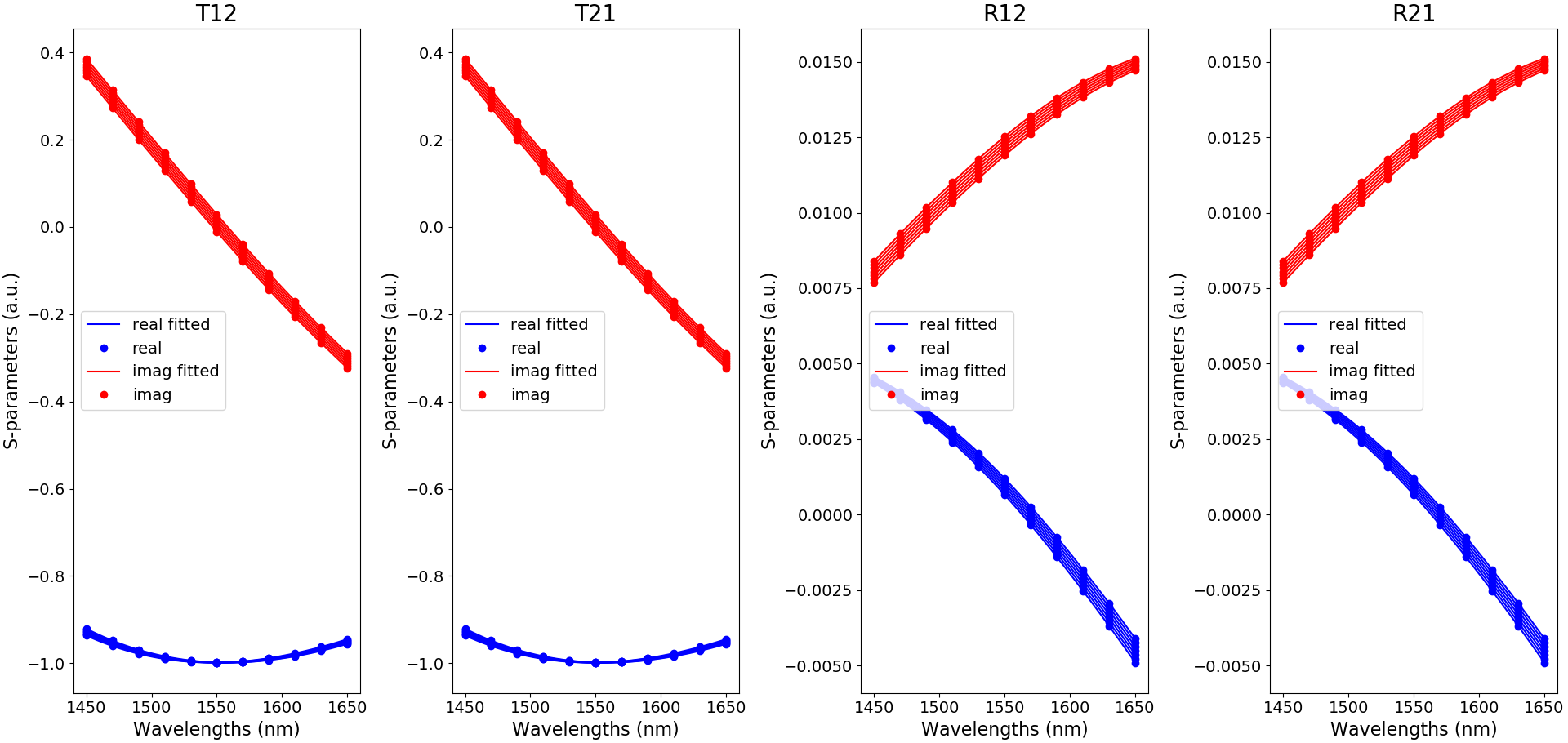
../../../_images/uc_mostsensitive_fitting.png — Fitting to the TE-polarized S matrix coefficients of the optimized unit cell configuration yielding the best temperature sensitivity

We have also now explicitly defined the bounds of the wavelength and temperature sweeps according to the specs of our application. When looking at the model_data folder, you will see that a new .txt file has been created for our optimized unit cell that contains the fitting data. You will also see that the configuration is added to the whats_there file.

Now that the unit cell is optimized to achieve high temperature sensitivity and its circuit model created, we can finally start generating the resulting WBG layout and circuit model.