1. Introduction
First of all, what do we mean by optical modulation? Well, suppose you have an electrical sine wave with frequency \(\omega_{rf}\) and that it is encoded with a data stream.
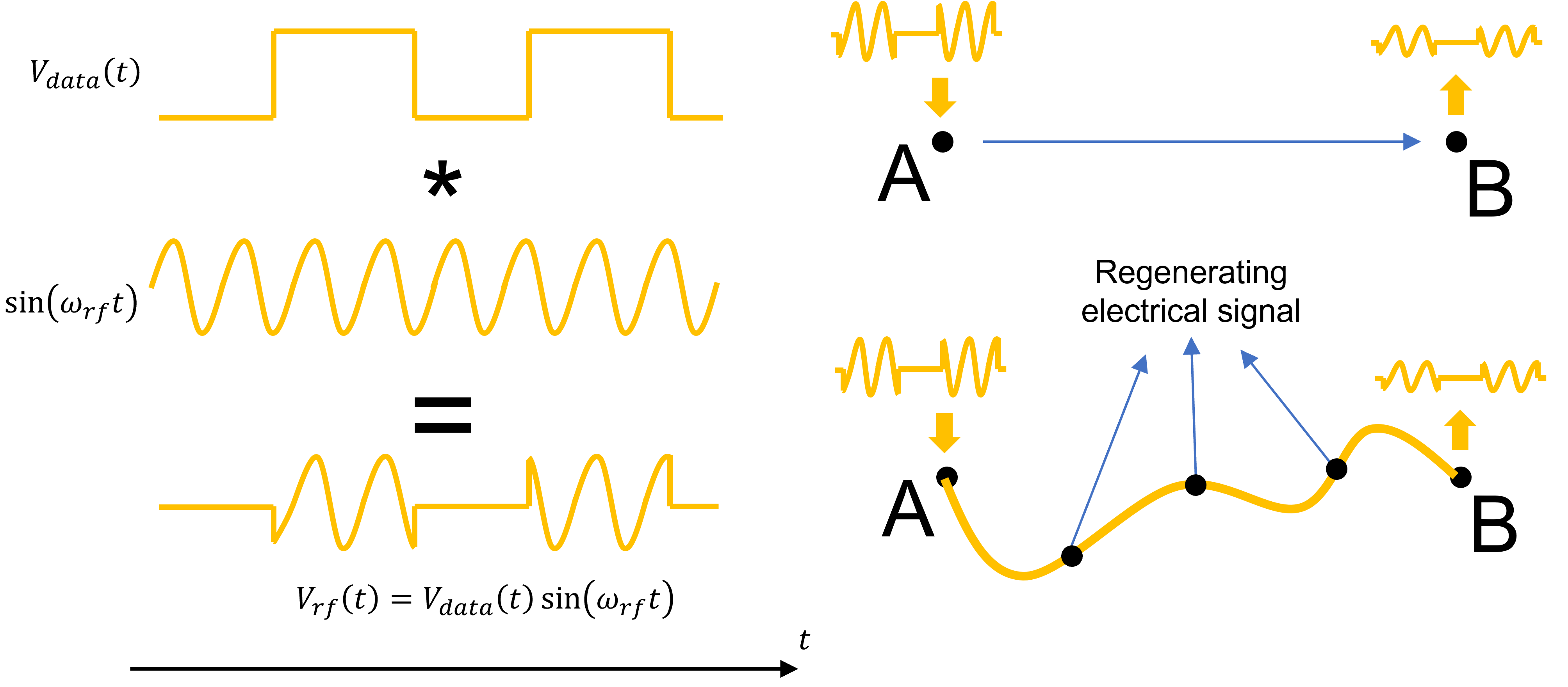
Data stream encoded on an electrical sine wave with frequency \(\omega_{rf}\), and how it can be transported from point A to B.
To transport this data stream from point A to point B, one needs an electrical cable. However, as we have briefly touched upon in the introduction, signal degradation is a big problem in electrical cables due to the very large losses the electrical signals experience in these cables. This means that when sending a signal from point A to point B, the electrical signal needs to be regenerated (or cleaned up) an increasing amount of times as the distance between these points increases. When the frequency of the electrical signal \(\omega_{rf}\) also increases in order to be able to encode more data, the problem becomes even worse and the amount of points where regeneration of the electrical signal is required increases even more. To avoid these limitations, we use optical fibers instead of electrical cables to transmit the data between points A and B. The optical signal losses in the optical fibers are several orders of magnitude smaller than the electrical signal losses in the electrical cables, and hence, no signal generation is required over several hundreds of kilometers instead of several meters for the electrical cables. The question however is: how can we change that electrical signal carrying the data into an optical one?
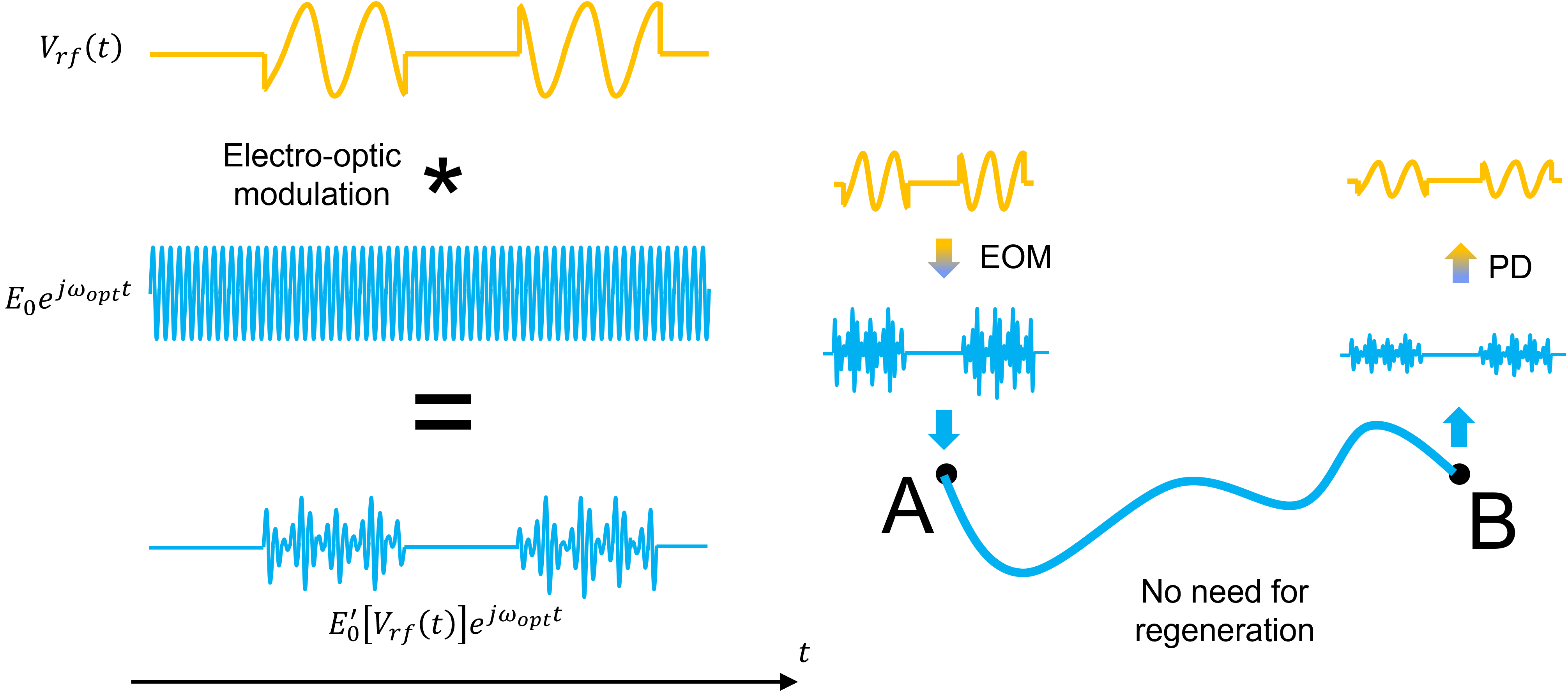
Illustration of amplitude modulation of a CW optical signal with the aforementioned high speed electric signal that we want to transport from point A to B. On the right, we illustrate that the electrical signal is modulated on the optical wave at point A, the modulated optical signal is transported over the optical fiber, and the original electrical data is retrieved through a photodiode (PD) at point B.
To do so, we employ an electro-optic modulator (EOM). This device dynamically changes, certain physical parameters of the material using the electric signal carrying the data. If a continuous wave (CW) optical signal (i.e. a wave that is a pure sinusoid with a certain optical frequency \(\omega_{opt}\) or optical wavelength \(2\pi c/\omega_{opt}\), with \(c\) the speed of light) travels through that material, its properties will change as well. The properties of the optical wave that we can change are
the phase, by electrically changing the refractive index of the material,and
the amplitude, by electrically changing the optical losses in the material.
The process of changing these parameters with an electric signal is called, not surprisingly, electro-optic modulation. However, just as encoding the data onto the optical wave through an EOM is important, it is equally important to be able to retrieve the data from that modulated optical signal, or be able to demodulate the optical signal back into the electrical domain. Since converting an optical signal back into an electrical signal can only be done using a photo-detector (PD), only amplitude modulated light can be used. This means that we either need to use an electro-absorption modulator (EAMs) or convert the phase modulated signal from an electro-optic phase modulator (EOPM) into an amplitude modulated signal. The latter option is often more advantageous than the former option considering EOPMs typically have a lower insertion loss than EAMs and considering there is a wider variety of integrated EOPMs than integrated EAMs.
And this is where the MZM comes in handy: the MZM is a device used to create an amplitude modulated optical signal from a phase modulated optical wave. It is based on an interferometric structure, called a Mach-Zehnder interferometer (MZI).
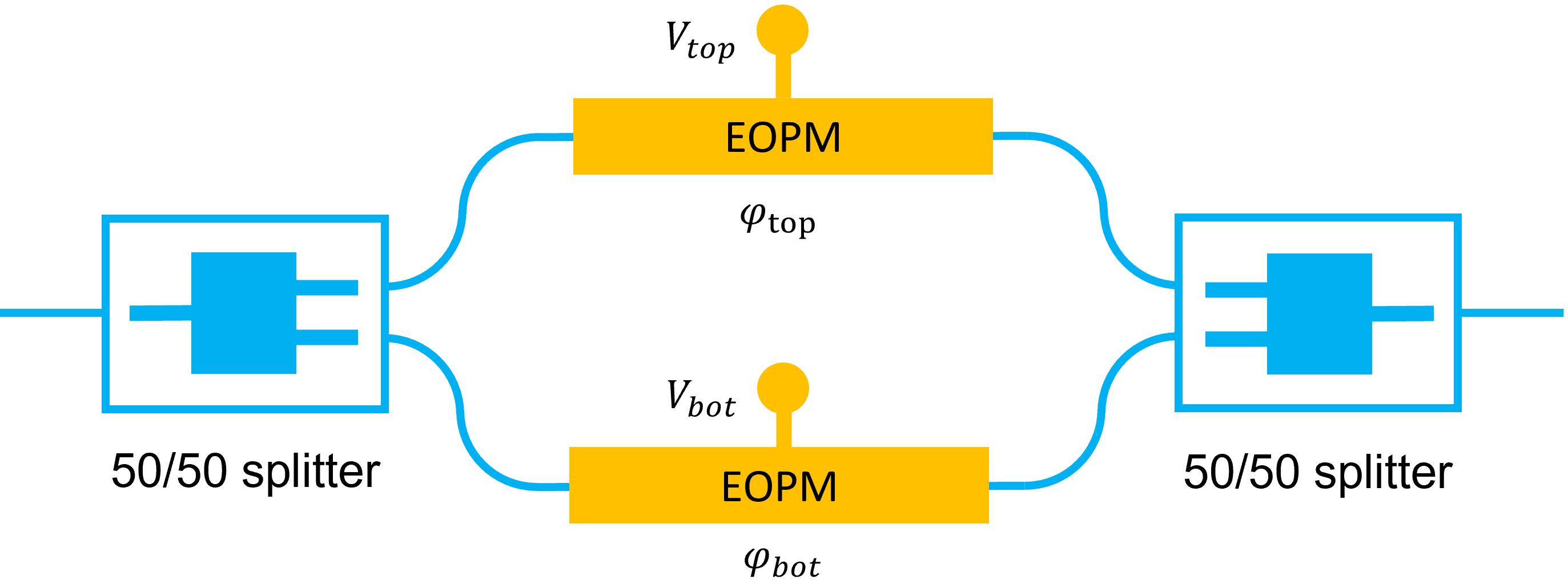
Schematic representation of a Mach-Zehnder interferometer (MZI), containing an EOPM in each arm, giving each arm a certain phase.
In an MZI, the incoming optical wave is first equally split over two arms using a 50/50 splitter and is then recombined by a second 50/50 splitter. When the two beams are recombined, two different scenarios can take place:
If the two separate paths have equal optical length or phase, the split beams are in phase when they recombine and constructive interference is achieved.
If the optical lengths or phases of the two paths are different, the split beams will have different relative phase when they recombine. This gives rise to destructive interference.
Therefore, depending on the relative phase difference acquired by the split beams while traveling along the two separate paths, the light is recombined either more efficiently or less. As a result, the optical power at the output port will change depending on the phase difference. In the following image, the output power of an MZI is plotted as a function of the phase difference \(\Delta\Phi\), when the input optical power is 1 mW.
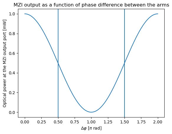
Transmitted power at the MZI output port as a function of the phase difference \(\Delta\varphi\) between the arms.
Phase shifting the optical wave in the top arm relative to that in the bottom arm thus results in a changing optical output power. If we assume that only the top arm contains an EOPM, the total phase difference will only be determined by the phase shift induced in the top arm. But if both arms contain an EOPM, the total phase difference will be determined by the difference in phase shifts induced by the EOPMs. How much of a phase shift is induced by the EOPM for a certain applied voltage will be discussed in the next subsection.
1.1. Performance of the modulator
An important parameter of the EOPM is the efficiency: how much phase shift do you get per applied voltage? The EOPM efficiency will depend on the physical process you’re using to achieve the electro-optic modulation (more on that in the next sections), and on the EOPM length (longer EOPMs result in more interaction between the optical and electric signals).
1.1.1. First property: \(V_\pi\)
To quantify the EOPM efficiency, we look at the property commonly referred to as the \(V_\pi\), which indicates the voltage difference between the voltage for which no light is transmitted (full destructive interference when the beams recombine) and the closest voltage for which all the light is transmitted (full constructive interference when the beams recombine). For full destructive interference, there is a phase difference of \(\pi\) between the MZM arms, while for full constructive interference, there is no phase difference between the MZM arms. Hence, the phase difference between those two states is \(\pi\) and this is where the name \(V_\pi\) comes from: it is the voltage for which you achieve a \(\pi\) phase shift. A smaller \(V_\pi\) thus means the same optical output power swing can be achieved at lower voltage differences, thus making the modulator more efficient. With the \(V_\pi\) known, then for the MZM configuration where only the top arm contains an EOPM and where both MZM arms have the same length, the phase shift induced by an input voltage \(V_{top}\) is given by \(\phi_{mod}=\pi V_{top}/V_{\pi}\). Consequently, the optical power at the MZM’s output port for a given input optical power \(P_{in}\) can be calculated as:
Plotting \(P_{out}/P_{in}\) as a function of \(V_{top}\) gives the aforementioned MZM characteristic (illustrated for \(V_\pi=1 V\)):
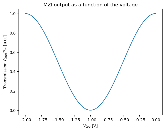
Transmitted power at the output port of an MZI that only has an EOPM in the top arm, as a function of the voltage \(V_{top}\) applied to the EOPM.
1.1.2. Second property: Quadrature bias point
Naturally, having a small \(V_\pi\) is not the only important aspect to achieve efficient modulation. Also biasing the MZM properly is key to achieve this goal. To understand what that means, realise that in a lot of cases, the high speed electrical signal is not only a sinusoid carrying a data signal, but also has a DC bias added to it:
\(V_{in}(t)=V_{bias}+V_{data}(t)\sin(\omega_{rf}t)\)
Why is this necessary? Well one reason could be, as explained in the next section, that the modulator is more efficient (i.e. has a lower \(V_\pi\)) at particular values of \(V_{bias}\). But there is another, more important reason. Let’s look again at the MZM characteristic:
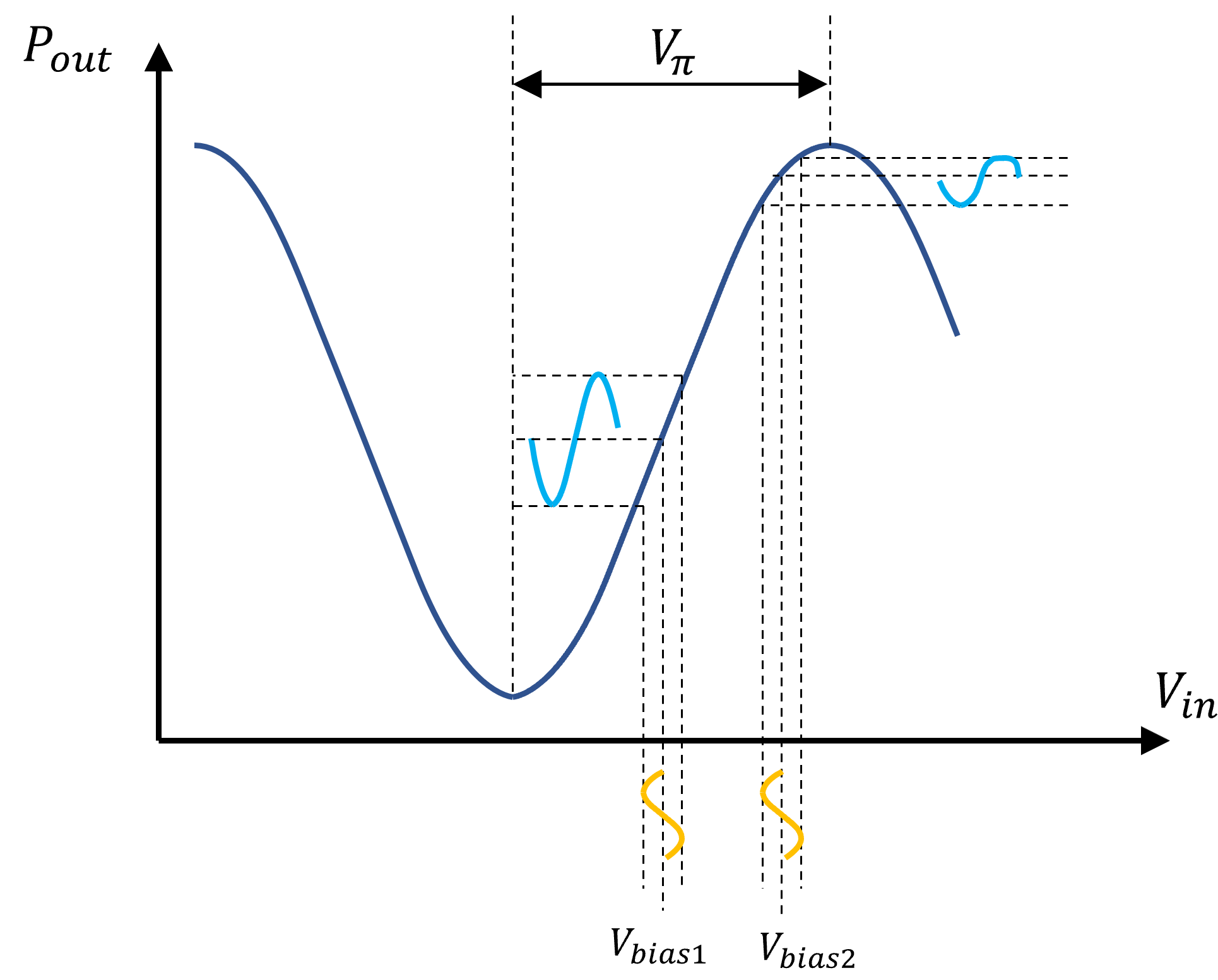
Illustration that the bias point heavily influences the modulation efficiency as well as the signal distortion. \(V_{bias1}\) corresponds to quadrature bias as it is located exactly in the middle between the two extrema of the characteristic.
Suppose that we put \(V_{bias}\) right in the middle between the maximum and minimum. If we now apply a small sinusoidal electrical signal on top of that, the optical output power will have a certain sinusoidal swing that can be estimated graphically as illustrated on the figure. But if we place \(V_{bias}\) closer to either the maximum or the minimum transmission, we see that the optical output power swing is much less pronounced than in the previous case, where \(V_{bias}\) is right in the middle between the two extrema. Moreover, we also see signal distortions, i.e. the optical output power is not a ‘clean’ sinusoid anymore, due to the increasingly nonlinear relation between \(P_{out}/P_{in}\) and \(V_{in}\) closer to the minimum or maximum. As such, setting \(V_{bias}\) exactly in the middle between the two extrema will optimise both the efficiency and linearity of the MZM. This point is called the quadrature bias point, because it corresponds to a \(\pi/2\) phase shift between the MZM arms.
1.2. Modulator design choices
So in the previous subsection, we introduced two important MZM properties: the \(V_\pi\) and the quadrature bias point. Both properties can be optimised using a careful design of the MZM layout. Let’s focus on \(V_\pi\) first and then discuss optimising the MZM design in regards to the quadrature bias point afterwards.
1.2.1. Design choices to optimise \(V_\pi\)
First of all, we can lower the \(V_\pi\) of the full MZM with a factor of 2 ‘artificially’ by driving the modulator in the push-pull configuration (see below).
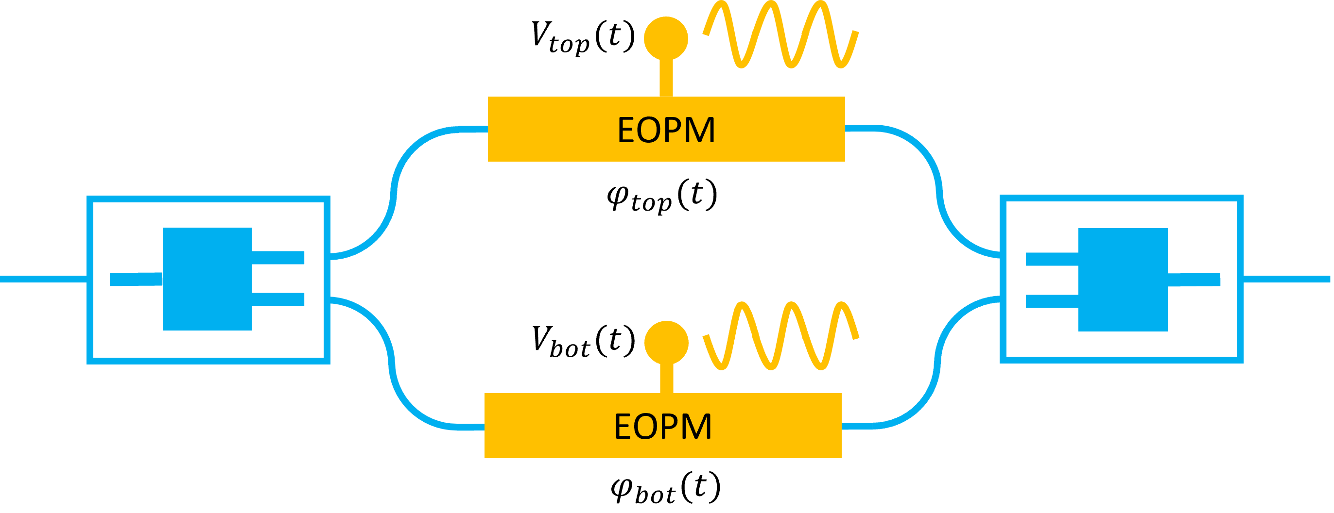
MZM in the push-pull configuration, whereby the same RF signal is applied to both MZM arms, albeit with a phase difference of \(\pi\).
In the push-pull configuration, the same RF signal is applied to both arms of the MZM, although with a \(\pi\) phase difference:
From this, we can derive the following equation for the output power:
with \(\Delta V^{dc}=V_{top}^{dc}-V_{bot}^{dc}\). Clearly, the push-pull configuration reduces the RF driving signal \(V_{data}(t)\sin(\omega_{rf}t)\) with a factor of two. Although one can’t really make the argument that the modulator is more efficient (after all, you now need two driving signals instead of one), a reduced driving voltage still benefits the MZM in other ways such as an improved linearity.
What will actually physically change \(V_\pi\), is the EOPM length. A longer EOPM length will result in more interaction between the optical signal and the material whose optical properties have been changed by the electrical signal. Needless to say, there are limitations on the maximum length of the EOPM due to the limited chip area. Apart from a limited chip area, another factor that limits the maximum length of the EOPM is the bandwidth. If you want to be able to modulate light with a high-speed electrical signal having a center frequency of \(\omega_{rf}\), you need to have a bandwidth larger than \(\omega_{rf}\). Since the EOPM length is inversely proportional with the bandwidth, long EOPMs will have a smaller bandwidth than short ones. So, while you do have a larger electro-optic interaction from having longer EOPMs, it is sadly counteracted by the decrease in bandwidth. This means that you don’t gain much in terms of modulation efficiency - if you gain anything at all - when the electrical signals you want to modulate the light with a frequency that exceeds the modulator bandwidth. There are EOPM designs that circumvent this issue somewhat, such as the travelling-wave EOPMs (TW-EOPMs). In these devices, the high-speed electric signals behave as propagating waves similar to how the optical signals behave in an optical waveguide - the difference being that these high speed electrical signals propagate in the the metal lines placed along the optical waveguide. To ensure proper electro-optic interaction and a high modulation efficiency at high frequencies, the optical and electrical waves co-propagate, i.e. both waves have the same propagation direction. Nevertheless, long TW-EOPMs still suffer from bandwidth issues as the RF wave degrades increasingly along the metal lines for higher frequencies. Either way, the TW-EOPMs will be the design used for this application example, although we limit ourselves by describing them as an RC circuit in the models as we will see in the next section. However, it should be stressed that Luceda IPKISS can deal with the more complex and accurate models that do take into account the travelling wave aspect of these devices, but this is beyond the scope of this application example.
1.2.2. Design choices to optimise the quadrature bias point
The other MZM property we introduced is the quadrature bias point. While biasing the modulator at quadrature is done by changing the DC bias voltage of the RF signal, it can also be done by creating an asymmetric MZM, where the phsycial length of the MZM arms is different. By carefully changing the difference in length between the MZM arms, a phase difference of \(\pi/2\) between the two arms can be achieved without the need for a DC bias voltage. Nevertheless, a DC bias voltage will always be required considering the fact that the EOPMs fully operate in reverse bias (meaning that the voltage needs to be negative over the active section of the EOPM at all times) and considering \(V_\pi\) is often dependent on \(V_{bias}\). Also, in real life, due to typical fabrication errors, the actual length difference between the MZM arms differs slightly from design specifications. As such, to achieve the optimal operation on-chip, we will always add additional EOPMs. Since these EOPMs are solely used for DC biasing, an RF signal will not be applied to them. EOPMs that are solely used for DC biasing are also called phase shifters, and we will refer to them as such from now on.
By separating the DC biasing from the actual high-speed modulation, one can optimize the MZM layout by using different types of EOPMs, or EOPMs that rely on different physical processes to modulate light. For example, one can use heater phase shifters for the DC biasing, while using carrier injection/depletion based EOPMs for the high-speed modulation. Changing the temperature changes the refractive index of the material through the material’s thermo-optic effect. While this is a particularly strong effect, i.e. even a slight temperature change can result in a large phase change, it is also a very slow effect (in the order of milliseconds). But since the phase shifters operate at DC voltages, the speed is no issue, and thus the heaters are perfectly suited for the DC biasing. And since the phase changes induced by carrier injection/depletion in carrier-based EOPMs happen on much shorter time scales (below 1 ns), these devices can be then used for the high-speed modulation.
1.2.3. Final MZM configuration
By taking all of this into account, we end up with the following MZM configuration:
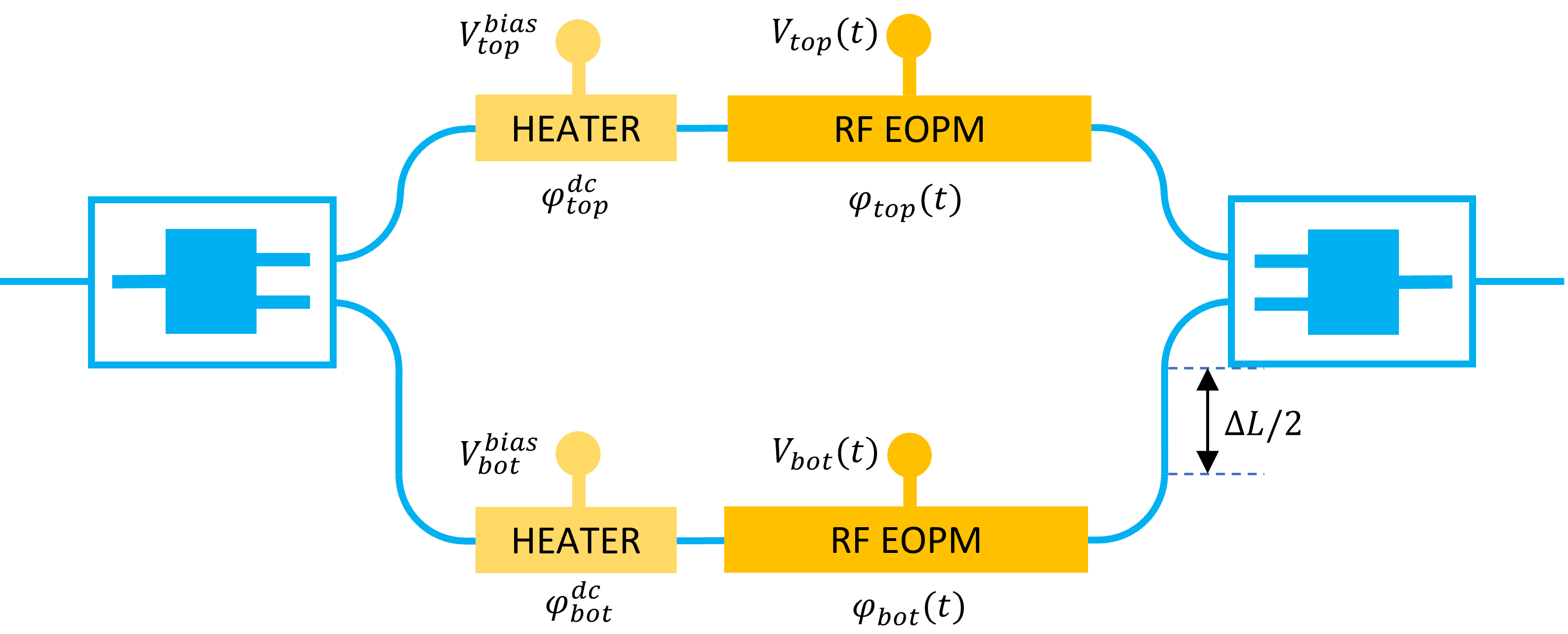
Schematic representation of a general MZM with a phase shifter and a heater on each arm and whereby the arms have a different length.
In the next two sections, you will learn how to implement and simulate the key building blocks of the MZM:
a carrier injection/depletion-based EOPM,
a phase shifter based on a heated waveguide.
For more details on the design and the compact model of the heater we will use for the MZM, have a look at the documentation of the heater included in SiFab: Heaters.