Y-branch
SiFab contains two Y-branches:
YBranch: a fully parametric Y-branch, with one input and two outputs.
YBranchOptimized: a 1x2 Y-branch optimized using inverse design, with locked properties.
The section Simulation and regeneration of the data files explains how to simulate and regenerate the simulation data of a Y-branch.
YBranch
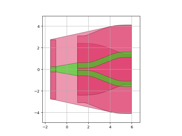
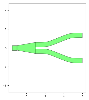
This is a Y-branch with fully customisable layout.
This class has a circuit model where the following parameters can be provided to perform a circuit simulation of the Y-branch: center_wavelength, transmission, reflection_in and reflection_out.
Reference
Click on the name of the component below to see the complete PCell reference.
Splitter in the form of a Y-branch with 1 input and 2 outputs. |
Example
from si_fab import all as pdk

length = 5.0

y_branch = pdk.YBranch(bend_length=length, bend_height=1.0)
lv = y_branch.Layout()
lv.visualize()
Model
For the Y-branch, we use the following model:
where \(t\) is the transmission (through), \(r_1\) is the reflection at the input and \(r_2\) is the reflection at the output. \(t\), \(r_1\), \(r_2\) are dispersive with respect to wavelength.
Simulation
Stand-alone simulations of the YBranch PCell can be performed by applying the simulation recipe of the Y-branch on a parametric layout.
Usually, this is done to explore the component behaviour when the parameters are changed, or to optimize it.
As simulations can take time to complete, it is best to organise and save all the simulation results in one folder for later inspection.
This allows us to run long simulations once and process the data later.
Reference
Click on the name of the function below to see the complete PCell reference.
|
It simulates a Y-branch using the link to ANSYS Lumerical FDTD and returns the transmission and reflection. |
Example
from si_fab import all as pdk
from si_fab.components.y_branch.simulation.simulate_lumerical import simulate_ybranch_by_lumerical_fdtd
from ipkiss3.simulation.circuit.utils import convert_smatrix_units
from ipkiss3 import all as i3
import os
inspect = False # Inspect the simulation
resimulate = True # Resimulate
plot = True # Plot the simulation result
wl_start = 1.5
wl_end = 1.6
n_points = 100
length = 5.0
project_folder = "./ybranch_sim" # Name of the project
smatrix_path = os.path.join(project_folder, "smatrix.s3p") # Path where the smatrix is saved
if not os.path.exists(project_folder):
os.mkdir(project_folder)
y_branch = pdk.YBranch(bend_length=length, bend_height=1.0)
lv = y_branch.Layout()
fig = lv.visualize()
fig.savefig(
os.path.join(project_folder, "ybranch_sim_layout.png"),
transparent=True,
bbox_inches="tight",
)
# Note that these simulation results are artificial results as they're based on fictional technology
# and components. They only serve demonstration purposes.
if resimulate:
smatrix = simulate_ybranch_by_lumerical_fdtd(
layout=lv,
project_folder=project_folder,
wavelengths=(wl_start, wl_end, n_points),
inspect=inspect,
)
smatrix.to_touchstone(smatrix_path)
if plot:
smatrix = convert_smatrix_units(
i3.device_sim.SMatrix1DSweep.from_touchstone(smatrix_path),
to_unit="um",
)
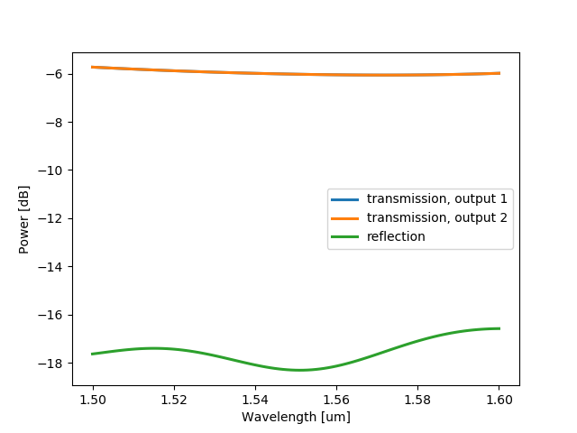
smatrix.visualize(
term_pairs=[
("in1", "out1"), # transmission 1
("in1", "out2"), # transmission 2
("in1", "in1"), # reflection
],
scale="dB",
show=False,
save_name=os.path.join(project_folder, "model.png"),
)
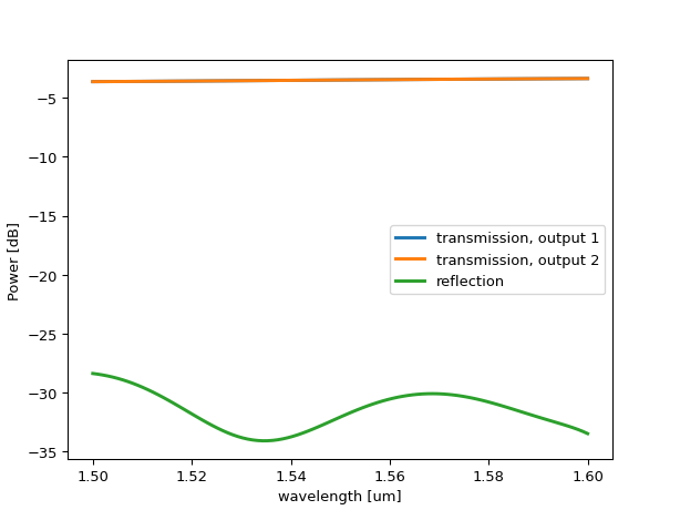
YBranchOptimized
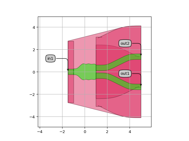
This Y-branch inherits from YBranch.
All the properties are locked, because the layout has been optimized to obtain maximum transmission at 1550 nm wavelength.
The optimization of this component has been performed using an inverse design simulation with Ansys Lumerical FDTD.
The layout was re-implemented in IPKISS.
We also provide a simulation recipe that launches a validation simulation using the Luceda Link for Ansys Lumerical.
After the simulation, a fitting is performed of the transmission and reflections as a function of wavelength.
The fitting coefficients for \(t\), \(r1\), \(r2\) are stored and used by Caphe (IPKISS’ circuit simulator) to calculate the S-matrix and perform a circuit simulation.
Reference
Click on the name of the component below to see the complete PCell reference.
This Y-branch is the result of an inverse optimization process performed using Ansys Lumerical FDTD. |
Example
from si_fab import all as pdk
import numpy as np


y_branch = pdk.YBranchOptimized()
lv = y_branch.Layout()
lv.visualize(annotate=True)

cm = y_branch.CircuitModel()
wavs = np.linspace(1.5, 1.6, 100)
smatrix = cm.get_smatrix(wavelengths=wavs)
smatrix.visualize(
    term_pairs=[
        ("in1", "out1"),  # transmission 1
        ("in1", "out2"),  # transmission 2
        ("in1", "in1"),  # reflection
    ],
    scale="dB",
)
Simulation and regeneration of the data files
The simulation data of YBranchOptimized (or of any other Y-branch class you optimize yourself) obtained with Lumerical FDTD can be regenerated.
This can be done with the regenerate_ybranch() function using the script regenerate_ybranch_optimized.py contained in si_fab/components/y_branch/regeneration.
The user can specify the following options:
ybranch_class: the Y-branch to regenerate. The name should not contain parentheses ().wavelengths: Tuple representing the wavelength range for the simulation and for the plots. The tuple must be in the format (min, max, number of points).center_wavelength: the center wavelength of the component.resimulate: boolean. If True, the Y-branch will be simulated at all thewavelengths. A fitting of the transmission as a function of wavelength is performed and the results are stored in a file in data/component_name.json.plot: boolean. If True, it plots the results of the simulation.
Reference
Click on the name of the functions below to see the complete API reference of the simulation and regeneration recipes.
|
It simulates a Y-branch using the link to ANSYS Lumerical FDTD and returns the transmission and reflection. |
|
It regenerates the simulation fitting data and/or the plots of the optimized Y-splitter. |
Note
The above simulation results are artificial results as they’re based on fictional technology and components. These only serve demonstration purposes.