6. Calculating coupler coefficients
A MZI Lattice filter uses a set of identical delay lines, or delay lines that are an integer multiple of a unit delay \(L\) which resembles just like in discrete Finite Impulse Response (FIR) filter.
Mathematical tools have been developed to approximate an ideal filter function on a discrete set of zeros that can be synthesized through an FIR filter.
The zeros coming out of such a design method that can be translated into a set of coupling coefficients through a method put forward by Jinguji and Kawashi in the paper Synthesis of Coherent Two-Port Lattice-Form Optical Delay-Line Circuit
A special class of FIR filters are Optical Half-Band Filters which have the property of having a symmetric passband and crossband. This property makes them very practical to be used in cascaded demultiplexers. The half-band lattice filters uses delays of both \(L\) and \(2L\). This approach can raise the order of the filter with fewer directional couplers.
In Optical Half-Band Filters the coupling coefficients of optical half band filters are computed for a Chebychev window and a window yielding a maximally flat passband as a function of center wavelength and trace template.
In the code below, we use the results from the paper to calculate the coupling coefficients and delay lengths.
from si_fab import all as pdk
import numpy as np
from pteam_library_si_fab.components.mux2.pcell.lattice_utils import (
    get_mzi_delta_length_from_fsr,
    get_length_pi,
    flip_couplings_and_delays,
)

tt = pdk.SiWireWaveguideTemplate()
# Series of power couplings and delay lengths for optical halfband filters
center_wavelength = 1.5
length = get_mzi_delta_length_from_fsr(trace_template=tt, center_wavelength=center_wavelength, fsr=0.01)
length_pi = get_length_pi(trace_template=tt, center_wavelength=center_wavelength)

# Maximally Flat

# N = 2
power_couplings_2 = np.sin(np.array([0.0833, 0.333, 0.25]) * np.pi) ** 2
delay_lengths_2 = [2 * length - length_pi, length]
print(power_couplings_2)
# N = 3
power_couplings_3 = np.sin(np.array([0.4664, 0.1591, 0.3755, 0.25]) * np.pi) ** 2
delay_lengths_3 = [2 * length, 2 * length - length_pi, length]
print(power_couplings_3)
# N = 4
power_couplings_4 = np.sin(np.array([0.3720, 0.2860, 0.4547, 0.1187, 0.25]) * np.pi) ** 2
delay_lengths_4 = [2 * length - length_pi, 2 * length, 2 * length - length_pi, length]
print(power_couplings_4)

# Chebychev
# N = 4
power_couplings_4c = np.sin(np.array([0.3498, 0.2448, 0.4186, 0.0797, 0.25]) * np.pi) ** 2
delay_lengths_4c = [2 * length - length_pi, 2 * length, 2 * length - length_pi, length]
print(power_couplings_4c)
[ 0.06693495  0.74909255  0.5       ]
[ 0.98889893  0.22970362  0.85466236  0.5       ]
[ 0.84682665  0.61213538  0.97988305  0.13273214  0.5       ]
[ 0.79338407  0.48366662  0.93601755  0.0613934   0.5       ]
6.1. Transforming the filter
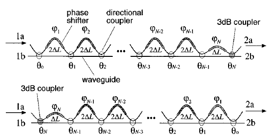
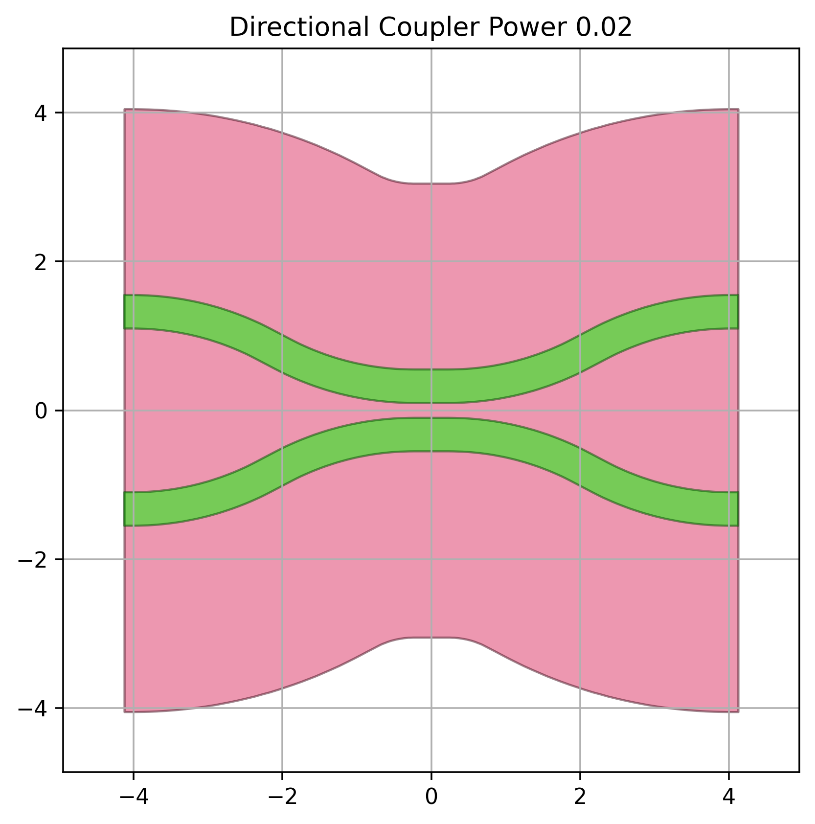
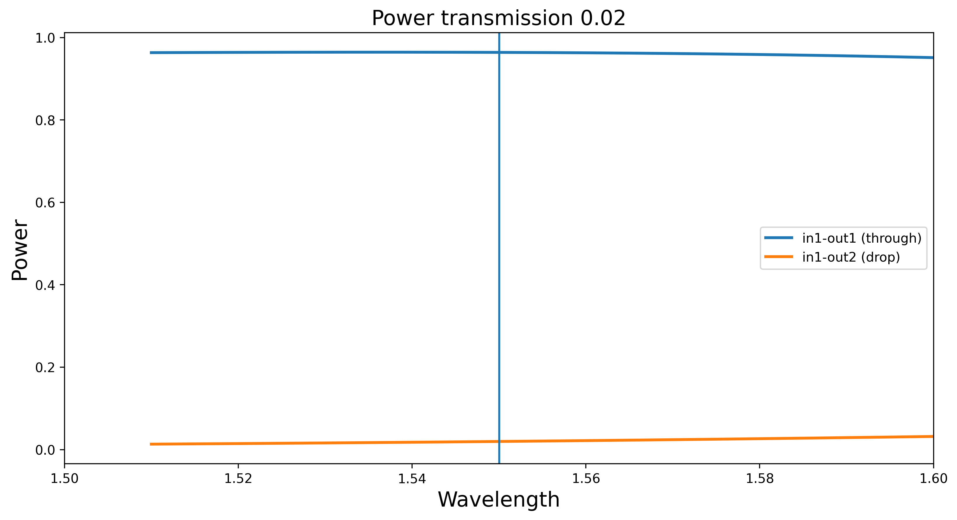
When the required directional coupler power \(p\) couplings that come out of the synthesis are close to 1 the directional couplers that implement such a coupling tend to be longer and more dispersive. This is shown in the figures below demonstrating a directional couplers with length 0.02 and 0.98.
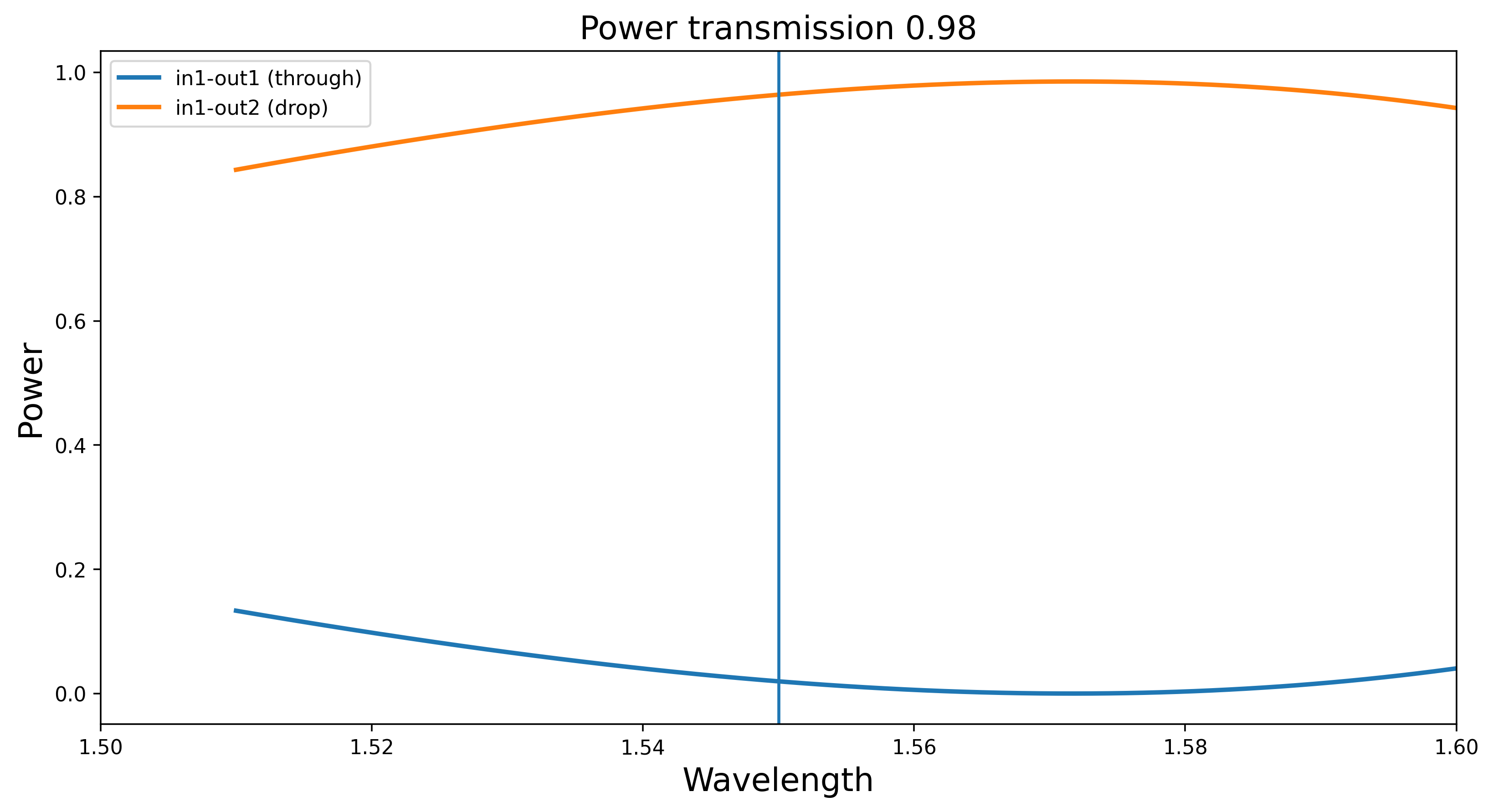
In such situations it is advisable to use the adjoint coupling power \(1-p\) and modify the delay lengths in such a way that the global transfer functions remains the same.
Without going into details, we have implemented such a function flip_couplings_and_delays that given a set of power_couplings, delay_lengths and the length_pi,
length of a waveguide yielding to a \(\pi\)-phase shift one can compute a new set of coupling factors and delay lengths where the couplers coupling \(p_i\) will be \(1-p_i\) for all i in flips.
# Flipping the coefficients and delay lengths
new_couplings, new_delays = flip_couplings_and_delays(
    couplings=power_couplings_4c,
    delay_lengths=delay_lengths_4c,
    length_pi=length_pi,
    flips=[0, 2],
)

print(
    f"""
original_couplings {power_couplings_4c}
new_couplings {new_couplings}
original_delays {delay_lengths_4c}
new_delays {new_delays}
"""  # fmt: skip
)
original_couplings [0.79338407 0.48366662 0.93601755 0.0613934  0.5       ]
new_couplings [0.20661592613749635, 0.4836666245332381, 0.06398244751668469, 0.06139339649771525, 0.5000000000000001]
original_delays [106.44044832613518, 106.75077033291691, 106.44044832613518, 53.37538516645846]
new_delays [-106.13012631935345, -106.44044832613518, 106.13012631935345, 53.37538516645846]
The longer directional couplers with coupling 0.79 and 0.94 have now been replaced by couplers with coupling 0.21 and 0.06.