Mach-Zehnder interferometer
The Mach-Zehnder interferometer (MZI) we are going to design is composed of:
One input fiber grating coupler
One Y-branch splitter
One broadband directional coupler
Two output fiber grating couplers
Two waveguide arms (left and right) connecting the two outputs of the splitter to the two inputs of the directional coupler
Two waveguides connecting the two outputs of the directional coupler to the two output fiber grating couplers
IPKISS integrates the different aspects of photonic design into one framework, where you can define your component once as a parametric cell (PCell) and then use it throughout the whole design process, allowing to tightly link layout and simulations.
Therefore, in order to easily create and manipulate the MZI that we need, we are going to create a PCell.
This PCell inherits from i3.Circuit, a class that makes it is easy to place and connect components together to achieve the final circuit.
PCell Properties
The first step is to define the PCell properties, which will be used to design the MZI. One aspect to pay attention to is the right arm of the MZI. Depending on the length of this arm, the result of the MZI simulation will change. Therefore, we need to be able to control the shape of this arm when we instantiate the MZI PCell, without touching the code inside the PCell itself.
The PCell has the following accessible properties:
delay_length: This determines the difference in length between the right (longer) and left (shorter) arm of the MZI.bend_radius: Here, we assign the value of the bend radius used for the waveguide routes.fgc: The PCell of the fiber grating coupler to be used. The default value isEBeamGCTE1550from the Luceda PDK for SiEPIC.splitter: The PCell of the splitter to be used. The default value isEBeamY1550from the Luceda PDK for SiEPIC.dir_coupler: The PCell of the directional coupler to be used. The default value isEBeamBDCTE1550from the Luceda PDK for SiEPIC.
Below is the code that defines the PCell properties.
class MZI(i3.Circuit):
    bend_radius = i3.PositiveNumberProperty(default=5.0, doc="Bend radius of the waveguides")

    fgc = i3.ChildCellProperty(doc="PCell for the fiber grating coupler")
    splitter = i3.ChildCellProperty(doc="PCell for the Y-Branch")
    dir_coupler = i3.ChildCellProperty(doc="PCell for the directional coupler")

    delay_length = i3.PositiveNumberProperty(default=60.0, doc="length difference between the arms of the MZI")

    def _default_fgc(self):
        return pdk.EbeamGCTE1550()

    def _default_splitter(self):
        return pdk.EbeamY1550()

    def _default_dir_coupler(self):
        return pdk.EbeamBDCTE1550()
Cells, placement and connections
The next step is to define a list of cells that will be instantiated. We need three fiber grating couplers, one splitter and one directional coupler.
    def _default_specs(self):
        specs = [
            i3.Inst(["fgc_1", "fgc_2", "fgc_3"], self.fgc),
            i3.Inst("yb", self.splitter),
            i3.Inst("dc", self.dir_coupler),
        ]
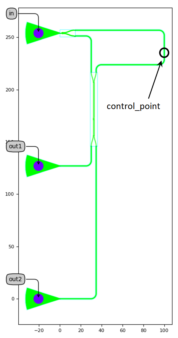
We place the input port of the bottom fiber grating coupler at the origin (0.0, 0.0). We then create an array of fiber grating couplers by placing the second grating coupler 127 um above the first, and the third 127 um above the second. Finally, we place the directional coupler relative to the output ports of the Y-branch splitter and rotate it 90 degrees.
luceda-academy/training/topical_training/siepic_mzi_dc_sweep/mzi_pcell.pydef _default_specs(self): specs = [ i3.Inst(["fgc_1", "fgc_2", "fgc_3"], self.fgc), i3.Inst("yb", self.splitter), i3.Inst("dc", self.dir_coupler), ] fgc_spacing_y = 127.0 specs += [ i3.Place("fgc_1:opt1", (0, 0)), i3.Place("fgc_2:opt1", (0.0, fgc_spacing_y), relative_to="fgc_1:opt1"), i3.Place("fgc_3:opt1", (0.0, fgc_spacing_y), relative_to="fgc_2:opt1"), i3.Place("dc:opt1", (20.0, -40.0), angle=90, relative_to="yb:opt2"), i3.Join("fgc_3:opt1", "yb:opt1"), ] specs += [ i3.ConnectManhattan( [ ("yb:opt3", "dc:opt2", "yb_opt3_to_dc_opt2"), ("dc:opt4", "fgc_2:opt1", "dc_opt4_to_fgc_2_opt1"), ("dc:opt3", "fgc_1:opt1", "dc_opt3_to_fgc_1_opt1"), ] ), i3.ConnectManhattan( "yb:opt2", "dc:opt1", "yb_opt2_to_dc_opt1", control_points=[i3.V(120.0, flexible=True)], match_path_length=i3.MatchLength(reference="yb_opt3_to_dc_opt2", delta=self.delay_length), ), ] return specs
The connections between the instances are defined differently depending on whether we connect them end-to-end or use a waveguide connector:
For end-to-end connections, we use
i3.Join. Here, we use this for the connection between the input fiber grating coupler and the splitter:To connect components using waveguide connectors, we use connectors (
i3.Connector). Here, we specify the type of connector used between the desired ports together with other useful information, such as the bend radius of the waveguides.
Components that are placed end-to-end using i3.Join are automatically placed by IPKISS to ensure that the connection requirement is satisfied.
In the case of connections defined using connectors, this is not the case.
IPKISS only knows that these two components have to be connected and the waveguide connector will be generated depending on their position, which we need to specify ourselves.
The connections between the splitter (“yb:opt2/3”) and the directional coupler (“dc:opt1/2”) are performed using a Manhattan-type waveguide connector (i3.ConnectManhattan) and adding path length matching requirements within one of the connectors. This path length matching is defined by setting the “delay_length” parameter of one connector with reference to another waveguide connection.
In this case, the right arm of the MZI (second connection) is forced to be delay_length longer than the left one.
The desired length is achieved by shifting a flexible control point.
The value given to that control point on instantiation is an initial guess.
In general, there are often multiple solutions to the length-matching problem, and IPKISS will choose the one closest to the initial guess.
This way, we can control which one of the possible length-matched paths will be followed by the connector.
See i3.MatchLength for more information on length matching of Manhattan connectors.
Exposed ports
Our circuit is almost finished. All we need to do now is to define the names of the external ports we want to access. We will use these port names to plot the transmission when we perform the circuit simulation.
    def _default_exposed_ports(self):
        exposed_ports = {
            "fgc_3:fib1": "in",
            "fgc_2:fib1": "out1",
            "fgc_1:fib1": "out2",
        }
        return exposed_ports
Run the code
Open luceda-academy/training/topical_training/siepic_mzi_dc_sweep/mzi_pcell.py.
At the bottom of the file, the MZI is instantiated and simulated:
# Layout
mzi = MZI(
name="MZI",
delay_length=60.0,
bend_radius=5.0,
)
mzi_layout = mzi.Layout()
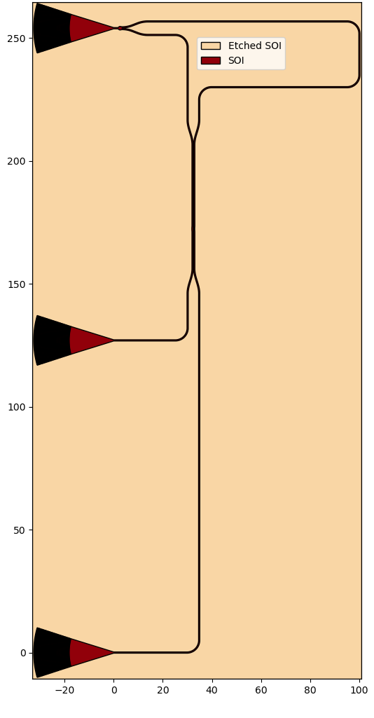
mzi_layout.visualize(annotate=True)
mzi_layout.visualize_2d()
mzi_layout.write_gdsii("mzi.gds")
# Circuit model
my_circuit_cm = mzi.CircuitModel()
wavelengths = np.linspace(1.52, 1.58, 4001)
S_total = my_circuit_cm.get_smatrix(wavelengths=wavelengths)
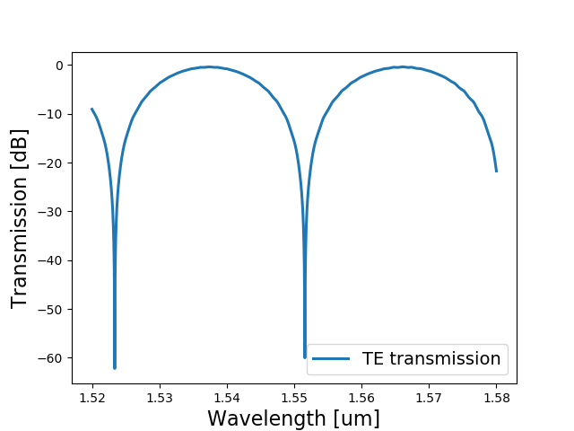
# Plotting
S_total.visualize(
term_pairs=[
("in:0", "out1:0"), # TE transmission 1
("in:0", "out2:0"), # TE transmission 2
],
scale="dB",
)
If you run the code, you will visualize the layout and the simulation of an MZI circuit for delay_length=60.0 and bend_radius=5.0.
Test your knowledge
Try to change the delay length and the bend radius to see how the simulation changes. What happens when the delay arm becomes longer? Why?