Design variations and hierarchical layout
The next step is to use the MZI PCell defined in the previous section to create a sweep of MZIs with different length of the right arm.
For this case, we will also use i3.Circuit to easily simulate each MZI that is part of our design to check their behavior.
When submitting designs to a foundry, more often than not you are allowed limited space to fit your designs.
To make sure that the design is not bigger than the allowed area, it is useful to use a frame.
The Luceda PDK for CORNERSTONE contains a PCell called DesignFrame, which can be used exactly for this purpose.
The height and width of this PCell are fixed to a width of 11.47 mm and a height of 15.45 mm.
This is quite generous so we will simply show how to fit on one small part of the frame.
Let’s now have a look at how we can define design variations using IPKISS. Open the file luceda-academy/training/topical_training/cornerstone_mzi_sweep/example_design_variations.py in your PyCharm project, so that you can follow along with the explanation.
Parameters for the MZI sweep
First of all, we define the parameters that we will use for the MZI sweep.
We want to design three different MZIs.
The right arm of each MZI will pass through a different coordinate in order to control its length.
We provide this coordinate to the MZI PCell using the control_point property.
The following parameters are defined at the beginning of the file:
control_points: A list of coordinates [(x1, y1), (x2, y2), (x3, y3)] that will be used to instantiate the MZI PCells of the three MZIs we want to design.bend_radius: The waveguide bend radius we will use for our designs.pos_xandpos_y: The x- and y-coordinates where we will place the bottom left fiber coupler of the first MZI. They are defined to be close to the bottom left corner of the design frame as the center of the design frame will be placed at the origin. This is why we use the large negative quantities of -5150 and -7700 micrometers.spacing_y: The vertical spacing between the fiber grating couplers of the three MZIs.
After defining these parameters, we create an empty insts dictionary and an empty specs list.
We will add to them all the cells that we want to instantiate and the placement specifications that we need to provide to i3.Circuit to create our final design.
# Parameters for the MZI sweep
control_points = [(100.0, 200.0), (200.0, 200.0), (300.0, 200.0)]
bend_radius = 80.0
pos_x = -5150
pos_y = -7700
spacing_y = 600

insts = dict()
specs = []
Design frame
Before designing the MZIs, it is good to have clear what are the boundaries for our design. We instantiate the design frame from the Luceda PDK for CORNERSTONE SiN, we add it to the instances dict and we place the bottom left corner at the origin.
# Create the design frame
design_frame = pdk.DesignFrame()

# Add the design frame to the instances dict and place it at (0.0, 0.0)
insts["design_frame"] = design_frame
specs.append(i3.Place("design_frame", (0.0, 0.0)))
MZI sweep
To create the MZI sweep, we use a practical for-loop over the list of control points.
Each time we instantiate an MZI with the correct control point, we add it to the dictionary of instances and place it at the coordinates (x0, y0).
For the first MZI, these are the coordinates we defined in the initial parameters.
For each following MZI, the value of y0 is increased by the value in spacing_y.
For our own reference, after each MZI is instantiated, we calculate the delay length between the two arms of the MZI and print it.
Very important!
Each time we instantiate an MZI, we have to assign a unique name.
Otherwise, the tree instantiated MZIs will be an exact copy of each other and changing the design of one of them will result in a change in all of them.
To make sure the names are all different, we use the for-loop counter ind to call them MZI0, MZI1, MZI2.
# Create the MZI sweep
for ind, cp in enumerate(control_points):
    mzi = MZI(
        name=f"MZI{ind}",
        control_point=cp,
        bend_radius=bend_radius,
    )

    # Calculate the actual delay length and print the results
    right_arm_length = mzi.get_connector_instances()[1].reference.trace_length()
    left_arm_length = mzi.get_connector_instances()[0].reference.trace_length()
    delay_length = right_arm_length - left_arm_length

    print(
        mzi.name,
        f"Delay length = {delay_length} um",
        f"Control points = {cp}",
    )

    mzi_cell_name = f"mzi{ind}"
    insts[mzi_cell_name] = mzi
    specs.append(i3.Place(mzi_cell_name, (pos_x, pos_y)))

    pos_y += spacing_y
Circuit design
We now create our circuit to be simulated using i3.Circuit.
Most of the heavy work is done.
We only need to instantiate a circuit cell that contains the instances and the placement specifications that we carefully defined before.
# Create the final design with i3.Circuit
circuit = i3.Circuit(
    name="CORNERSTONE_SiN_mathias",
    insts=insts,
    specs=specs,
)
Layout and circuit simulation
We can now instantiate the layout of the circuit to view it and save the layout of the final design to a GDS file:
# Layout
circuit_lv = circuit.Layout()
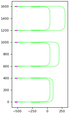
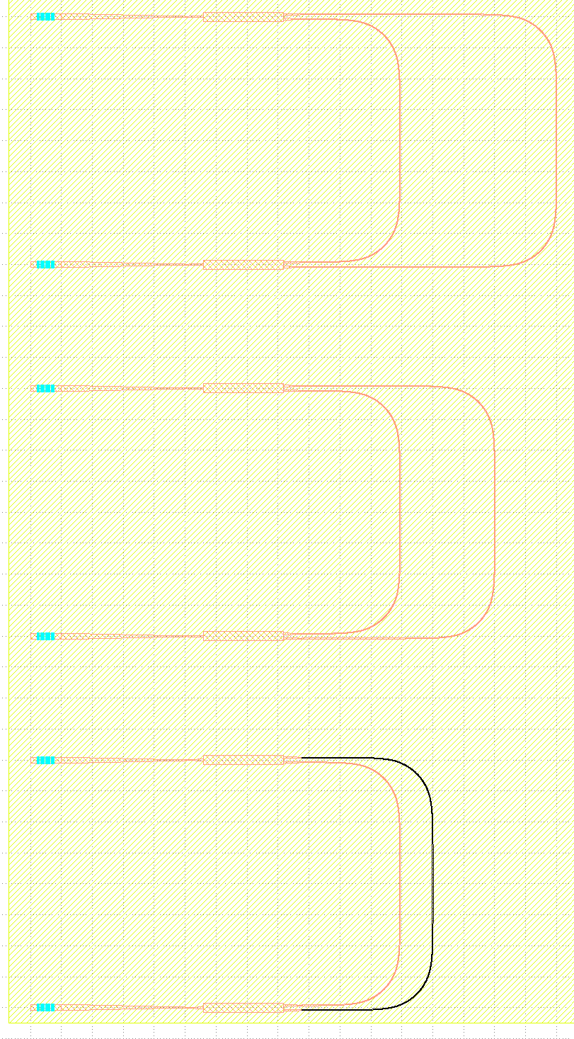
circuit_lv.visualize()
We show here the corner of the design frame we use for our design sweep:
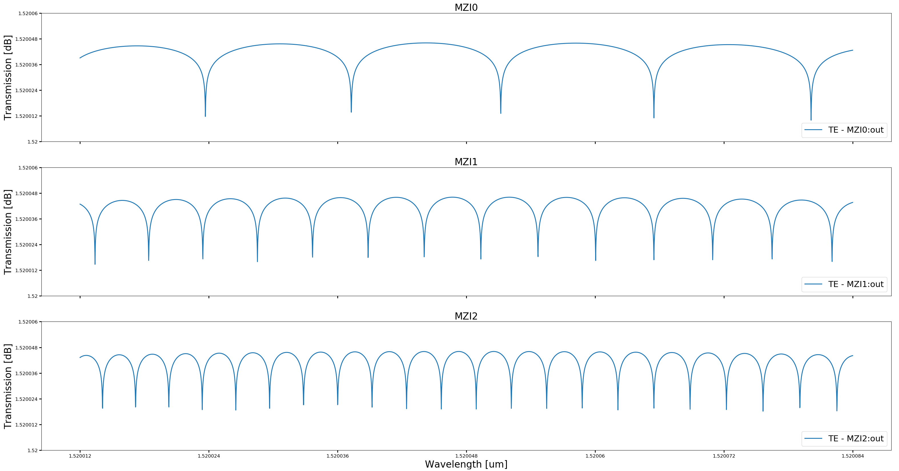
Next, we can extract the S-matrix and plot the results of the circuit simulation to visualize the behaviour of our MZIs:
# Circuit model
circuit_cm = circuit.CircuitModel()
wavelengths = np.linspace(1.52, 1.58, 5001)
S_total = circuit_cm.get_smatrix(wavelengths=wavelengths)

# Plotting
fig, axs = plt.subplots(3, sharex="all")

for ind, wav_sep in enumerate(control_points):
    S_total.visualize(term_pairs=[(f"mzi{ind}_in:0", f"mzi{ind}_out:0")], title=f"MZI{ind}", scale="dB")

print("Done")
Test your knowledge
Do these results satisfy your expectations? If not, change the control points to change the length of the right arm and check again the simulation.
Only a small fraction of the design frame is covered by this design sweep, how could you have a design sweep with 100 or even a 100 MZIs on the frame?