1.3. Adding fiber grating couplers

Adding fiber grating couplers to the MZI is now very simple. As done before with the Y-Branch and the waveguides, we need to:

1. Instantiate the correct fiber grating coupler from the Luceda PDK for SiEPIC

2. Add the grating couplers to the list of instances

3. Connect the grating couplers to the Y-Branches using i3.Join in specs

4. Flip the output grating coupler in specs

5. Update the external port names, as the vertical ports of the grating couplers are now the input and output of our circuit

luceda-academy/training/topical_training/siepic_mzi_ybranch/example_mzi_fgc.py

# 1. First, we instantiate the Y-branch from the SiEPICfab PDK.
splitter = pdk.EbeamY1550()
splitter_tt = splitter.Layout().ports["opt2"].trace_template

# 2. We instantiate the waveguides we will use for the arms of the MZI.
straight_length = 200.0
delay_length = 20.0
bump_angle = get_angle(straight_length=straight_length, delay_length=delay_length, initial_angle=10.0)

wg_straight = pdk.WaveguideStraight(wg_length=straight_length, trace_template=splitter_tt)
wg_bump = pdk.WaveguideBump(x_offset=straight_length, angle=bump_angle, trace_template=splitter_tt)

# 3. We instantiate the fiber grating coupler.
fgc = pdk.EbeamGCTE1550()
fgc.Layout().visualize(annotate=True)

# 4. We snap the ports to each other by using `i3.Join`.
# Other placement specifications define all the transformations that apply to each instance.
insts = {
    "yb_1": splitter,
    "yb_2": splitter,
    "wg_up": wg_bump,
    "wg_down": wg_straight,
    "fgc_1": fgc,
    "fgc_2": fgc,
}

# 5. We define specs, containing all the transformations that apply to each component.
specs = [
    i3.Join("fgc_1:opt1", "yb_1:opt1"),
    i3.Join("yb_1:opt2", "wg_up:pin1"),
    i3.Join("wg_up:pin2", "yb_2:opt2"),
    i3.Join("yb_1:opt3", "wg_down:pin1"),
    i3.Join("wg_down:pin2", "yb_2:opt3"),
    i3.Join("yb_2:opt1", "fgc_2:opt1"),
    i3.Place("yb_1:opt1", (0, 0)),
    i3.FlipH("yb_2"),
    i3.FlipH("fgc_2"),
]

# 6. We define the names of the exposed ports that we want to access.
exposed_port_names = {
    "fgc_1:fib1": "in",
    "fgc_2:fib1": "out",
}

# 7. We instantiate the i3.Circuit class to create the circuit.
mzi = i3.Circuit(
    name="mzi",
    insts=insts,
    specs=specs,
    exposed_ports=exposed_port_names,
)

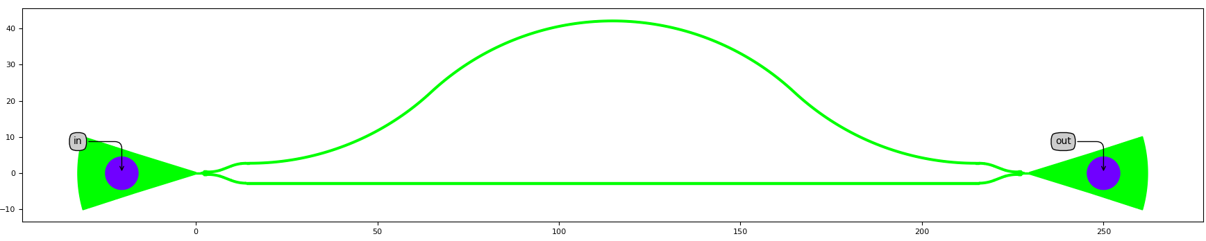
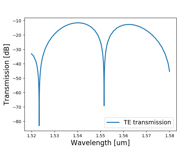
1.3.1. Layout and circuit simulation

We can now instantiate the layout of the circuit, visualize it, save it to GDSII and simulate it in IPKISS. You can see that the typical Gaussian behaviour of the fiber grating couplers is automatically taken into account in the result of the circuit simulation.

luceda-academy/training/topical_training/siepic_mzi_ybranch/example_mzi_fgc.py

# Layout
mzi_layout = mzi.Layout()
mzi_layout.visualize(annotate=True)
mzi_layout.write_gdsii("mzi_with_gratings.gds")

# Circuit model
mzi_cm = mzi.CircuitModel()
wavelengths = np.linspace(1.52, 1.58, 4001)
S_total = mzi_cm.get_smatrix(wavelengths=wavelengths)

# Plotting
plt.plot(wavelengths, i3.signal_power_dB(S_total["out:0", "in:0"]), "-", linewidth=2.2, label="TE transmission")
plt.xlabel("Wavelength [um]", fontsize=16)
plt.ylabel("Transmission [dB]", fontsize=16)
plt.legend(fontsize=14, loc=4)
plt.show()