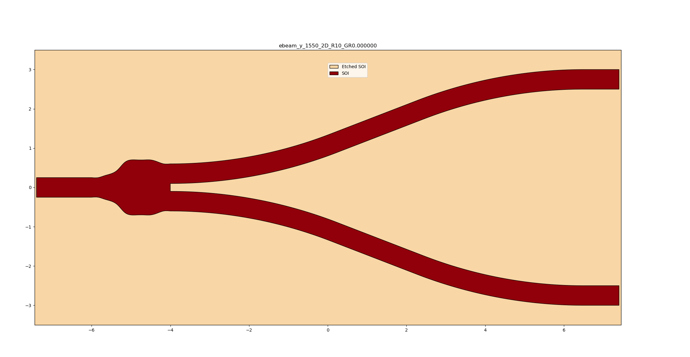
Y-Branch
The Y-Branch contained in the Luceda PDK for SiEPIC contains:
A layout view, which specifies what it looks like
A circuit model view, which specifies how it should be simulated
In the circuit model view, a previously defined compact model is used to tell Luceda IPKISS how to simulate this component. This compact model is defined separately from the component itself and can be found in pdks/siepic/ipkiss/siepic/cml/siepic_models.py.
class EbeamY1550CM(CompactModel):

    _model_type = 'python'
    parameters = ['through_coeff_TE', 'through_coeff_TM', 'refl_coeff_TE', 'refl_coeff_TM']
    states = []
    terms = [
        OpticalTerm(name='opt1', n_modes=2),
        OpticalTerm(name='opt2', n_modes=2),
        OpticalTerm(name='opt3', n_modes=2)
    ]

    def calculate_smatrix(parameters, env, S):
        if (env.wavelength < 1.5) or (env.wavelength > 1.58):
            raise Exception(
                "The wavelength is beyond the range of wavelength data points used for the Y-splitter model"
            )
        through_te_fit = polyval(parameters.through_coeff_TE, env.wavelength - 1.55)
        refl_te_fit = polyval(parameters.refl_coeff_TE, env.wavelength - 1.55)
        through_tm_fit = polyval(parameters.through_coeff_TM, env.wavelength - 1.55)
        refl_tm_fit = polyval(parameters.refl_coeff_TM, env.wavelength - 1.55)

        S['opt1:0', 'opt2:0'] = S['opt2:0', 'opt1:0'] = complex(through_te_fit)
        S['opt1:0', 'opt3:0'] = S['opt3:0', 'opt1:0'] = complex(through_te_fit)
        S['opt1:1', 'opt2:1'] = S['opt2:1', 'opt1:1'] = complex(through_tm_fit)
        S['opt1:1', 'opt3:1'] = S['opt3:1', 'opt1:1'] = complex(through_tm_fit)
        S['opt1:0', 'opt1:0'] = S['opt2:0', 'opt2:0'] = S['opt3:0', 'opt3:0'] = complex(refl_te_fit)
        S['opt1:1', 'opt1:1'] = S['opt2:1', 'opt2:1'] = S['opt3:1', 'opt3:1'] = complex(refl_tm_fit)
In this compact model, simulation data provided by the foundry, in this case obtained using simulations in Ansys Lumerical FDTD, is fitted and then used to calculate the elements of the S-matrix.
Layout
Before seeing how to simulate this component, let’s have a look at what the layout looks like. To do so, we perform the following steps:
We create a new file in our project. We call it ‘ybranch.py’ (you can find this file in training/topical_training/siepic_mzi_ybranch).
We start by including import statements: we need to import the Luceda PDK for SiEPIC, Luceda IPKISS and other Python libraries (numpy and pyplot) that we will need later to plot the simulation results.
We instantiate the component we want to visualize and we assign it to the variable
splitter.We instantiate the layout view of the Y-Branch with the command
splitter.Layout(). We assign it to a new variable which will contain the layout view:splitter_layout.Now we can apply different visualization command on the layout view to visualize the component:
Normal visualisation:
visualize()Virtual fabrication:
visualize_2d()Cross section:
cross_section().visualize(). Note: In the case of the cross section, you will also have to specify the line along which you want to visualize the cross section (see code below).
The code below contains all these steps, one after the other.
from siepic import all as pdk
from ipkiss3 import all as i3
import numpy as np

splitter = pdk.EbeamY1550()

# 1. Layout
splitter_layout = splitter.Layout()
splitter_layout.visualize(annotate=True)
splitter_layout.visualize_2d()
splitter_layout.cross_section(cross_section_path=i3.Shape([(-0.5, -1.5), (-0.5, 1.5)])).visualize()

Circuit simulation
Now that we’ve seen what the Y-Branch looks like, let’s learn how to simulate its behaviour.
First, we instantiate the circuit model view, similarly to what we did previously with the layout view. We assign the circuit model view to the variable
splitter_circuit. Keep in mind that the optimal operation wavelength of this component is 1.55 um. This is also clear from the name of the componentEBeamY1550.We define the wavelength range for the simulation, between 1.52 um and 1.58 um.
We calculate the S-matrix in the defined wavelength range.
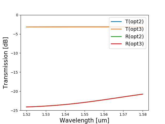
We plot the results, making sure to correctly specify the desired ports. In this case we are plotting:
S["opt2", "opt1"]: Transmission from port ‘opt1’ (input port) to port ‘opt2’ (top output port)S["opt3", "opt1"]: Transmission from port ‘opt1’ (input port) to port ‘opt3’ (bottom output port)S["opt2", "opt2"]: Reflection at port ‘opt2’ (top output port)S["opt3", "opt3"]: Reflection at port ‘opt3’ (bottom output port)
The code below contains all these steps, one after the other.
# 2. Circuit
splitter_circuit = splitter.CircuitModel()

# 3. Plotting
wavelengths = np.linspace(1.52, 1.58, 51)
S = splitter_circuit.get_smatrix(wavelengths=wavelengths)
S.visualize(
    term_pairs=[
        ("opt1", "opt2"),  # transmission opt2
        ("opt1", "opt3"),  # transmission opt3
        ("opt2", "opt2"),  # reflection opt2
        ("opt3", "opt3"),  # reflection opt3
    ],
    scale="dB",
    yrange=(-25, 0),
)
