4. Define a QCSE-based EAM component and an EAM-based circuit
In the final section, we will use the simulation and interpolation results from the previous section to construct a QCSE-based EAM component and an example circuit with an EAM on it. The layout of the component and circuit will be visualized, and the transmission spectrum of both the component and the circuit under different bias voltages will be shown.
4.1. Defining a QCSE-based EAM component
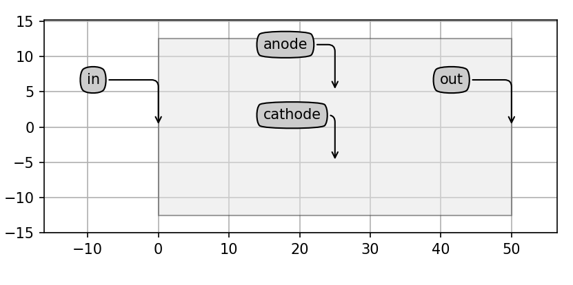
First, we define the class EAM_NN that inherits from i3.PCell. The shape of the QCSE-based EAM can be simplified to a rectangle in its layout, as it is a waveguide modulator. It has two optical ports: input and output. We define the QCSE-based EAM as a DC bias modulator, incorporating two electrical ports: anode and cathode.
The interpolation script described in the previous section will be applied to the circuit model of the QCSE-based EAM. We will instantiate several circuit model views, with bias voltages applied to the QCSE-based EAM taken from the list we created in the previous step.
from si_fab import all as pdk
import ipkiss3.all as i3
import numpy as np
import matplotlib.pyplot as plt
import os

"""
Parametrize a QCSE-EAM cell and its behavior model

We will create an EAM pcell based on our previous fitting data
"""

curdir = os.path.abspath(os.path.dirname(__file__))


# Class "EAM_NN" is the pcell of the EAM
class EAM_NN(i3.PCell):
    """
    Create the layout view of the EAM. The top view of the EAM is a rectangle,
    and it has 2 optical port and 2 electrical port
    """

    eam_length = i3.PositiveNumberProperty(doc="Length of the EAM [um]", default=50.0)

    class Layout(i3.LayoutView):
        """Create here the layout of this EAM"""

        def generate(self, layout):
            layout += i3.Rectangle(
                layer=i3.Layer(0), center=(self.eam_length / 2.0, 0.0), box_size=(self.eam_length, 25.0)
            )

            layout += i3.OpticalPort(
                name="in",
                position=(0, 0),
                angle=180,
                trace_template=pdk.SWG450(),
            )
            layout += i3.OpticalPort(
                name="out",
                position=(self.eam_length, 0),
                angle=0,
                trace_template=pdk.SWG450(),
            )
            layout += i3.ElectricalPort(
                name="anode",
                position=(self.eam_length / 2.0, 5),
                angle=90,
            )
            layout += i3.ElectricalPort(
                name="cathode",
                position=(self.eam_length / 2.0, -5),
                angle=-90,
            )
            return layout

    class Netlist(i3.NetlistFromLayout):
        pass

    class CircuitModel(i3.CircuitModelView):
        # Define all the properties for circuit model
        vbias_dc = i3.NumberProperty(doc="DC bias (only used for S parameters) [V]", default=2.0)

        def _generate_model(self):
            return EAMCompactModel(
                bias=self.vbias_dc,
            )  # compact model of EAM
The compact model contains the physical equations which describe the behavior of the component. We use the pickle module to load the interpolator we defined in the last chapter. We set the bias as a parameter in the CircuitModel, while we take the wavelength from environment when we simulate the component. The output of the interpolation result is the optical loss of the QCSE-based EAM.
class EAMCompactModel(i3.CompactModel):
    """Compact model for an electro-absorption modulator with the absorption modeled by nextnano. It is assumed the EAM
    has infinite bandwidth.
    For the calculation of S-parameters, we assume the voltage is constant and equal to `bias`,
    which is set via `vbias_dc` in the CircuitModelView of EAM_NN.
    """

    _model_type = "python"
    parameters = [
        "bias",
    ]

    states = []

    terms = [
        i3.OpticalTerm(name="in"),
        i3.OpticalTerm(name="out"),
        i3.ElectricalTerm(name="anode"),
        i3.ElectricalTerm(name="cathode"),
    ]

    def calculate_smatrix(parameters, env, S):
        wav = env.wavelength
        with open(os.path.join(curdir, "output_data", "interpolator.pkl"), "rb") as interp:
            import pickle

            interpolator = pickle.load(interp)
        loss_t = interpolator([parameters.bias, wav])
        S["in", "in"] = S["out", "out"] = 0.0
        S["in", "out"] = S["out", "in"] = 10.0 ** (-loss_t / 20.0)
4.2. Designing a QCSE-based EAM-based circuit
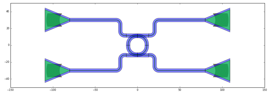
We design a circuit based on the EAM component described in the previous section. The circuit example will consist of an EAM and two grating couplers. The grating coupler cell FC_TE_1300 will be imported from the si_fab PDK.
We define a circuit class called EAMCircuit, and inherit from i3.Circuit.
""" Design a circuit based on QCSE-EAM pcell

This is the final step, we will demonstrate a circuit based on a EAM and connect to 2 grating coupler. """


class EAMCircuit(i3.Circuit):
    # 1. We define the properties of the EAM PCell.
    EAM = i3.ChildCellProperty()
    GC = i3.ChildCellProperty()
    spacing_x = i3.PositiveNumberProperty(default=200.0)
    spacing_y = i3.PositiveNumberProperty(default=50.0)

    def _default_EAM(self):
        return EAM_NN()

    def _default_GC(self):
        return pdk.FC_TE_1300()

    def _default_specs(self):
        # 2. We define instances that make up our circuit.
        # We have 2 grating coupler and 1 EAM.
        specs = [
            i3.Inst("EAM", self.EAM),
            i3.Inst(["fgc_in", "fgc_out"], self.GC),
        ]

        # 3. We define placement and routing specifications, containing all the transformations that apply
        # to each component, and connectors (list of connector object calls) and ports to be connected.

        sp_x = self.spacing_x

        specs += [
            i3.Place("EAM", (0, 0)),
            i3.Place("fgc_in:out", (-sp_x, 0.0), relative_to="EAM:in"),
            i3.Place("fgc_out:out", (sp_x, 0.0), angle=180.0, relative_to="EAM:out"),
            i3.ConnectManhattan("fgc_in:out", "EAM:in"),
            i3.ConnectManhattan("fgc_out:out", "EAM:out"),
        ]
        return specs

    # 4. We define the names of the external ports.
    def _default_exposed_ports(self):
        exposed_ports = {
            "fgc_in:vertical_in": "in",
            "fgc_out:vertical_in": "out",
        }
        return exposed_ports
4.3. Instantiating the QCSE-based EAM component and the EAM-based circuit
After defining the circuit, we instantiate it.
if __name__ == "__main__":
    # 1. We instantiate the EAM and the fiber grating coupler from siphog
    EAM = EAM_NN()
    GC = pdk.FC_TE_1300()

    # 2. We instantiate the EAM and visualize it
    EAM_layout = EAM.Layout()
    EAM_layout.visualize(annotate=True)
    wavelength_sweep = np.linspace(1.26, 1.36, 501)
    vbias_sweep = [1.0, 2.0, 3.0]

    for v_bias in vbias_sweep:
        EAM_biased = EAM.modified_copy()
        EAM_cm = EAM_biased.CircuitModel(vbias_dc=v_bias)
        S_total = EAM_cm.get_smatrix(wavelengths=wavelength_sweep)
        plt.plot(
            wavelength_sweep,
            -i3.signal_power_dB(S_total["out", "in"]),
            "-",
            linewidth=2.2,
            label=f"-{v_bias}V (Interpolation)",
        )

    plt.ylim(0, 2.5)
    plt.xlabel("Wavelength [um]", fontsize=16)
    plt.ylabel("Absorption [dB]", fontsize=16)
    plt.title("Absorption spectrum of QCSE-based EAM under different bias")
    plt.legend(fontsize=14, loc=4)
    plt.show()
First we instantiate the QCSE-based EAM component. The layout of the QCSE-based EAM is just made of a dummy layer with the available optical/electrical port information. We define the list of wavelengths and biases for which we simulate the QCSE-based EAM.

Layout visualization of the QCSE-based EAM
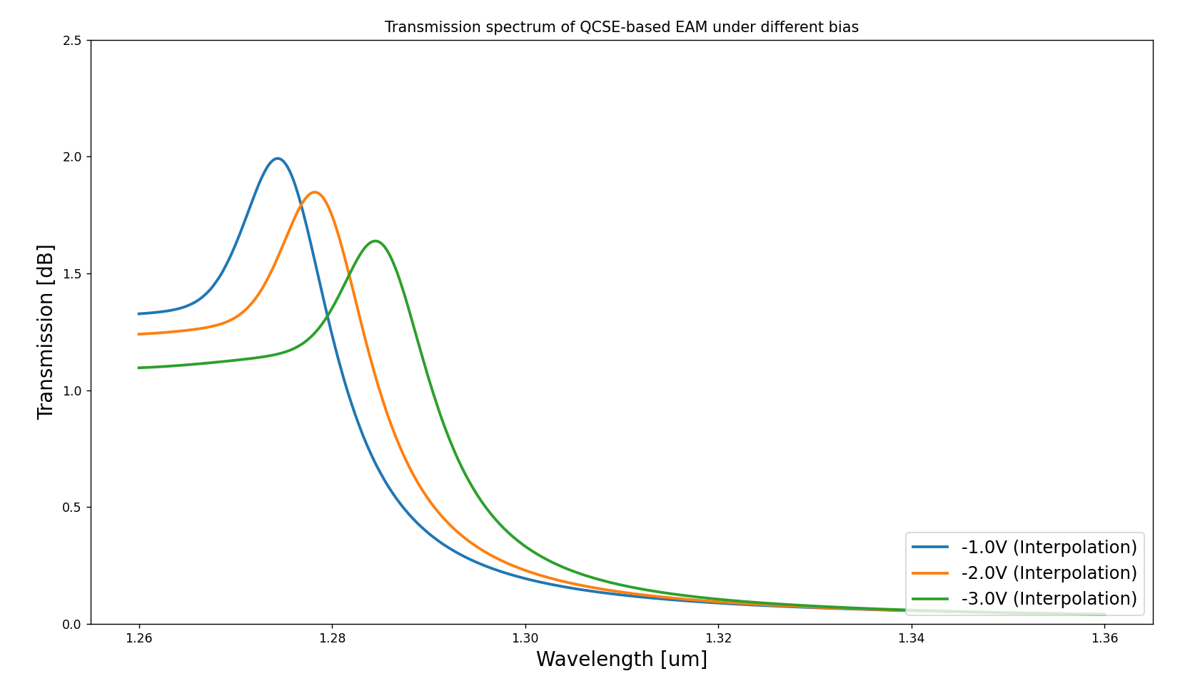
The simulation result is displayed in the image below. In this case, we interpolate the absorption spectrum of the QCSE-based EAM under bias voltages of -1V, -2V, and -3V. One can notice that as the bias increases, the exciton peak will have a red shift in the spectrum with lower absorption.

Absorption spectrum of the QCSE-based EAM under different interpolate bias voltage value
Next, we instantiate the QCSE-based EAM-based circuit.

Layout visualization of the QCSE-based EAM-based circuit
The wavelength is set in the O-band, ranging from 1.31 µm to 1.36 µm, with 501 steps, and the bias voltage is set from -1 V to -3 V, with 1 step.
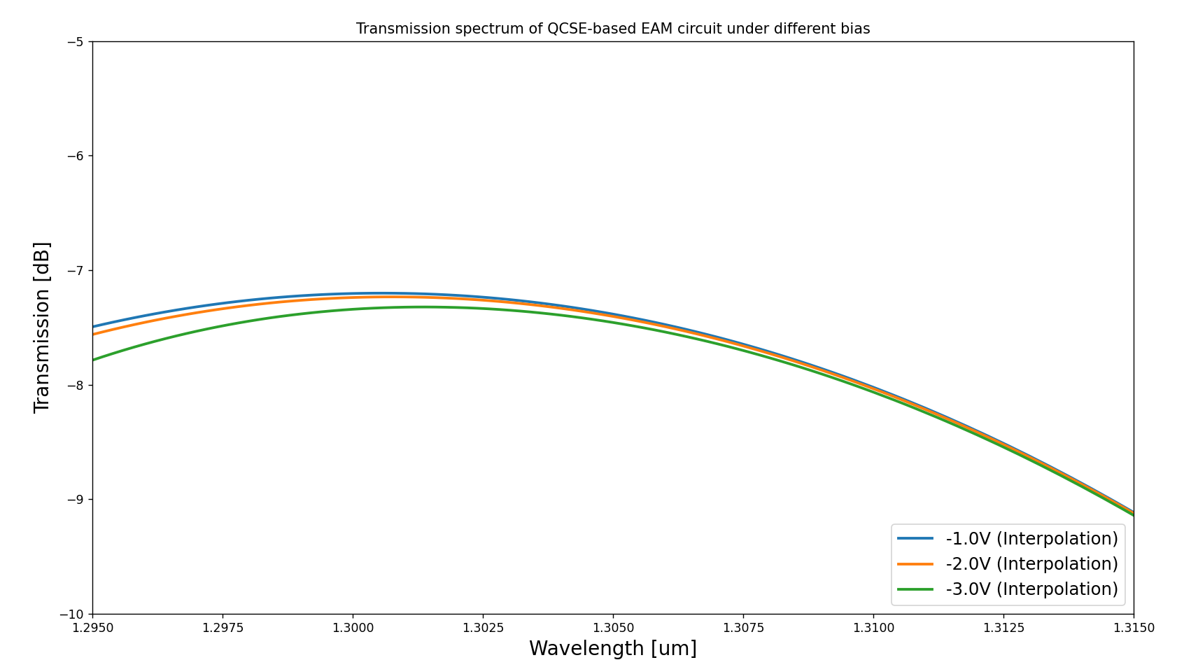
Subsequently, we plot the transmission spectrum of the circuit as a function of wavelength under different bias conditions.
Here, we zoom in to the wavelength range between 1295nm to 1315nm, since the modulation bandwidth is smaller compared to the bandwidth of the grating coupler.
The simulation results indicate that as the bias voltage increases, the transmission decreases, resulting in a red shift in the spectrum.

The interpolated transmission spectrum of the QCSE-based EAM-based circuit under different bias voltages