Circuit analyzer tutorial with Beneš switch
The Circuit Analyzer brings us one step closer to a first-time-right experience to tape-out by considering real world imperfections into PIC designs. With this module, users are able to assess worst- and best-case scenarios, evaluate design tolerances and estimate yield.
In this tutorial, we will guide you through the first steps of how to use the Circuit Analyzer (CA), breaking the process down into simple tasks. We will first focus on nominal simulation and then dive into CA with corner definition and corner analysis. There are advanced tutorials in our Luceda Academy that explore more complex features on top of the ones in this tutorial available in samples/circuit_analyzer.
Note
This tutorial assumes the reader has a basic understanding of compact models and nominal circuit simulation. If not, we advise reviewing documentation in our Academy prior to continuing. We will also use the following abbreviations: CA - circuit analyzer, CM - circuit model.
The structure is as follows:
Nominal simulation - using circuit simulation with CAPHE both in schematic with IPKISS Canvas and in code
Corner analysis - setting up the corners and performing analysis
Beneš switch and nominal simulation
To get started, we need a circuit to analyze. We will use an optical switch — namely, the Beneš switch, a well-known architecture in photonics. There are several architectures to implement switches, each with trade-offs depending on design goals such as power consumption or optical loss.
A basic \(2\times2\) Beneš switch is implemented by at least two directional couplers and a controllable heater connecting one of the arms.
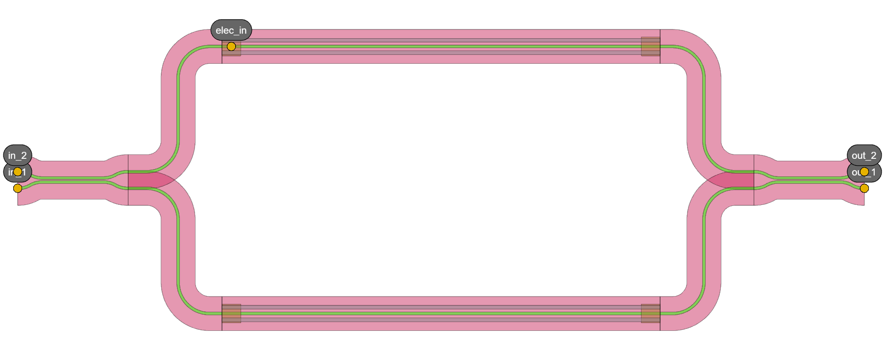
Beneš switch 2x2
In training/topical_training/circuit_analyzer_benes_switch/switch_4x4 script in our academy, you can find the code for this circuit. Using the default settings for the circuit (voltage difference between the two heaters is zero and MZIs are balanced), we expect that input light from one port 1/2 to be fully directed to the opposite output due to \(90^{\circ}\) phase shift introduced by the balanced beam splitters.
    start_wavelength: float = 1.45
    end_wavelength: float = 1.55
    n_wavelength_points: int = 501
    wavelengths = np.linspace(start_wavelength, end_wavelength, n_wavelength_points)

    benes_2x2 = Switch_MZI2x2()
    benes_2x2.Layout().visualize()
    s_total = benes_2x2.CircuitModel().get_smatrix(wavelengths=wavelengths)
    s_total.visualize(title="Beneš switch 2x2")
Which returns the following results, as expected:
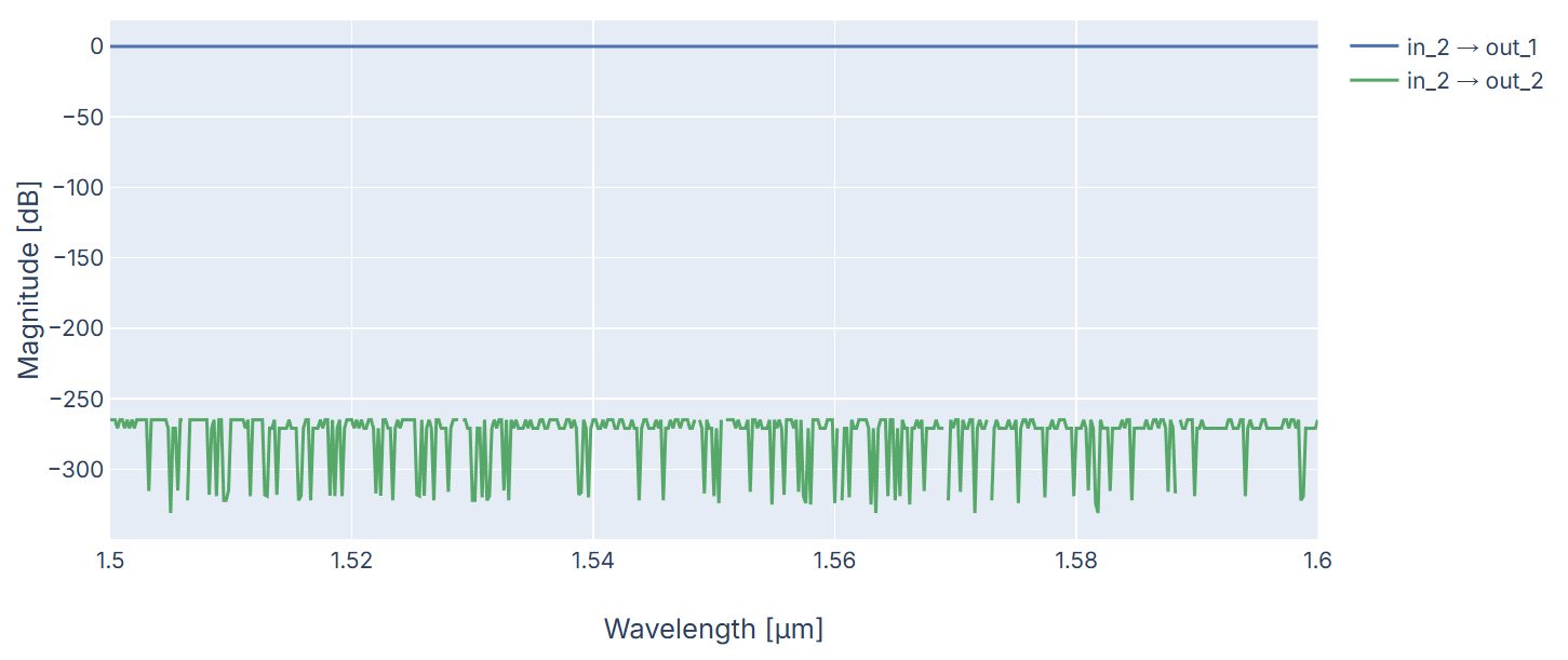
S-matrix results of the benes_2x2 for excitation at input 2
Scaling up to a \(4\times4\) Beneš switch, the circuit includes 6 MZIs - each with parametric voltage difference - and the respective connections. There are two points where the waveguides cross each other so we added Crossing components which is a component that allows to have these overlapping waveguides with low insertion loss, crosstalk and back-reflection. It results in the following circuit:
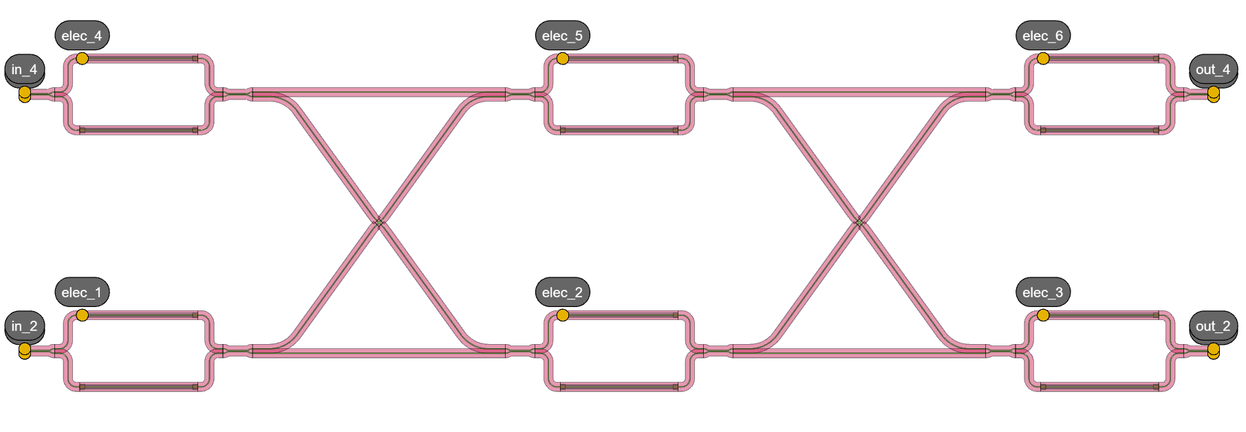
Benes switch 4x4
For simplicity, and as defined in the Beneš circuit script, let’s consider the voltage difference on all heaters set to:
\([2.416, 2.416, 2.416, 2.416, 2.416, 2.416]\)
This setting corresponds to a condition with no phase difference or delay between both arms of every switch. As a result, we expect light to enter and exit through the same numbered port (assuming a labeled and ordered port convention).
Similarly, and for the same wavelengths, we ran the following:
    benes_4x4 = Switch4x4_Benes(name="benes_4x4")
    benes_4x4.Layout().visualize()
    circuit_model_4x4 = benes_4x4.CircuitModel()

    S_total = circuit_model_4x4.get_smatrix(wavelengths=wavelengths)
    S_total.visualize(
        term_pairs=[("in_4", "out_1"), ("in_4", "out_2"), ("in_4", "out_3"), ("in_4", "out_4")],
        title="Beneš switch 4x4 - default vbias",
    )
Which returns the following results, as expected as well:
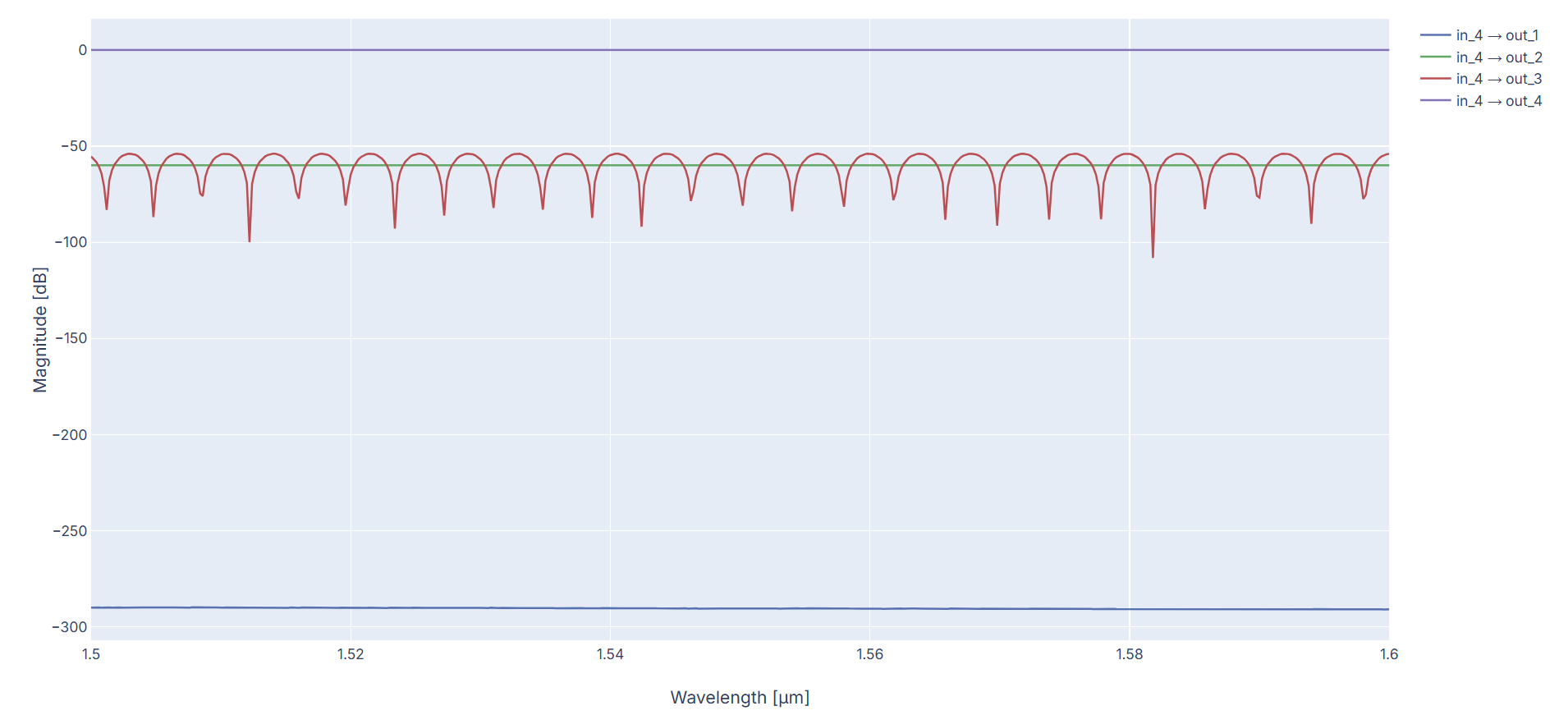
S-matrix results of the benes_4x4 for excitation at input 4
In order to run the circuit simulation, another option is to export the circuit to IPKISS Canvas, drag and drop the SMatrixSweep Codelet under generic_devices and press start button. With the Codelets section, we can find CornerAnalysis Codelet which can be used to run corner analysis as we will elaborate next.
Corner analysis
Now that we are aware of how the circuit works, let’s analyze its corners. Corners refer to values for our parameters in the circuit model that can deviate. They are commonly defined by two values along with the Nominal: Mininum and Maximum. The nominal is usually the default value of the parameter and the one used for the simulation as before, this is, under quasi-perfect conditions. The minimum and maximum corners define the range of how much the parameter can deviate from its default value due to any cause of variability.
For code readability and to work as a team on different aspects of the circuit, the corners are defined in a yaml file (models.yaml) which tells the CA what is modified in the CM and in a script models.py which tells the CA how they are modified. These files are in a ca_config folder which our Circuit Analyzer will read from and follow this structure:
ca_config/
├── models.py
└── models.yaml
Building your models.yaml and models.py file
In order to properly use corners, we select what corner properties we plan to include (can be anything and have any name) and then need to be aware of what parameters are part of the circuit so that we can translate them to a change in the Compact Model parameters.
When referring to parameters, let us start by clarifying that there are two types: (1) fabrication/performance parameters and (2) compact model parameters.
Fabrication/performance parameters can be those we see in schematic that are used for the Layout of our circuit such as length of a waveguide, spacing of two components or insertion loss. They can be anything and have a name of our choosing.
Compact model parameters are those needed to give to the component’s compact model to be able to calculate the scattering matrix.
The yaml file contains the fabrication/performance parameters and define its corners. The models.py file makes the correspondence to the compact model parameters; these need to be hand-in-hand with the models.py file for proper correspondence - it requires checking the arguments we give to the model in the PCell definition.
A very simple option is to use compact model parameters on both files and make a direct correspondence in models.py. The yaml file needs to follow the structure below:
version: 1
libraries:
    si_fab: # your library. Can be generic_devices as well or an added component in libraries/pteam_library...
        cells:
            HeatedWaveguide: # Your chosen component
                parameters:
                    loss:
                        doc: "loss in dB/m" #parameter description
                        default: 0.001
                        corners: [0.0006, 0.001, 0.002]
                generate_parameters: "models.heated_waveguide_parameters" # method were parameters are used
There, we defined the corners for our Beneš switch:
\([0.45, 0.5, 0.65]\) as cross_coupling in the directional coupler.
\([1.1, 1.2, 1.3]\) and \([0.0006, 0.001, 0.002]\) as width and loss in the heated waveguide respectively.
With this definition, the models.py will have the methods that take the corners and give them to the parameters of the compact models. We added a small multiplication to the loss parameter to match the units (defined per meter in yaml and per centimeter in CM).
def directional_coupler_parameters(self: library.DirectionalCouplerDC2.CircuitModel, **parameters):
    return {
        "cross_coupling": np.array([parameters["cross_coupling"]]),
    }


def heated_waveguide_parameters(self: pdk.HeatedWaveguide.CircuitModel, **parameters):
    return {
        "width": parameters["width"],
        "loss_db_per_cm": parameters["loss"] * 1e-2,
    }
To sum up the process so far:
Select a circuit. Ideally, run a simulation to become familiar with its behavior.
Define, in a yaml file, the parameters you want to vary in the circuit.
Write a models script where you make correspondence between the parameters defined in the yaml file and the compact models’ parameters.
After these 3 steps, we are ready to run corner analysis!
Running CA for Corner Analysis
Once the circuit is selected and the corners are defined, we are can start with a basic corner analysis.
We could analyze all corners via ca.corner_analysis_all_combinations,
which gives us a lot of information. However, this can become overwhelming — especially as the number of corners or circuit size increases.
If we have 2 parameters, each with the standard 3 values, we have 9 possibilities. For 4 parameters - slightly more realistic - it leads to 81 possibilities.
Therefore, we will use ca.corner_analysis which runs for a specific corner selection.
We chose matching “min”, “nominal” and “max” values for all parameters leading to 3 corner settings for each port pair:
The minimum corner corresponds to a corner value where all parameters have their minimum value.
The nominal value sets all parameters to their nominal value (which would be the default case).
The maximum corner corresponds to a corner value where all parameters have their maximum value.
from switch_4x4 import Switch4x4_Benes
from circuit_analyzer.fab_corner_variability import get_corners
import circuit_analyzer.all as ca

###########  Choosing the circuit and nominal simulation  ###########
benes_4x4.Layout().visualize()
end_wavelength: float = 1.55
    crns = get_corners(model_4x4)
    print(crns)  # we can print the corners to verify them

    corner_values = []
    for corner in ["min", "nominal", "max"]:
        kwargs = {c: corner for c in crns}
        smat = ca.corner_analysis(
            circuit_model=model_4x4,
            wavelengths=wavelengths,
            **kwargs,
        )
        corner_values.append(smat)
    ca.visualize_smatrices(
        title="Beneš switch min, nominal and max corners 4x4",
        smatrices=corner_values,
        term_pairs=[("in_4", "out_1"), ("in_4", "out_2"), ("in_4", "out_3"), ("in_4", "out_4")],
        smatrix_names=["min", "nominal", "max"],
    )

    all_corner_values = ca.corner_analysis_all_combinations(
With our S-matrix visualizer, we can easily edit the size of the s-matrix by excluding the ports of no interest (electrical in our case and keeping in_4 only) or select them as term_pairs in code. Changing the Layout theme to “Corner Analysis” once the visualizer opens, this results in the following visualization of the corners:
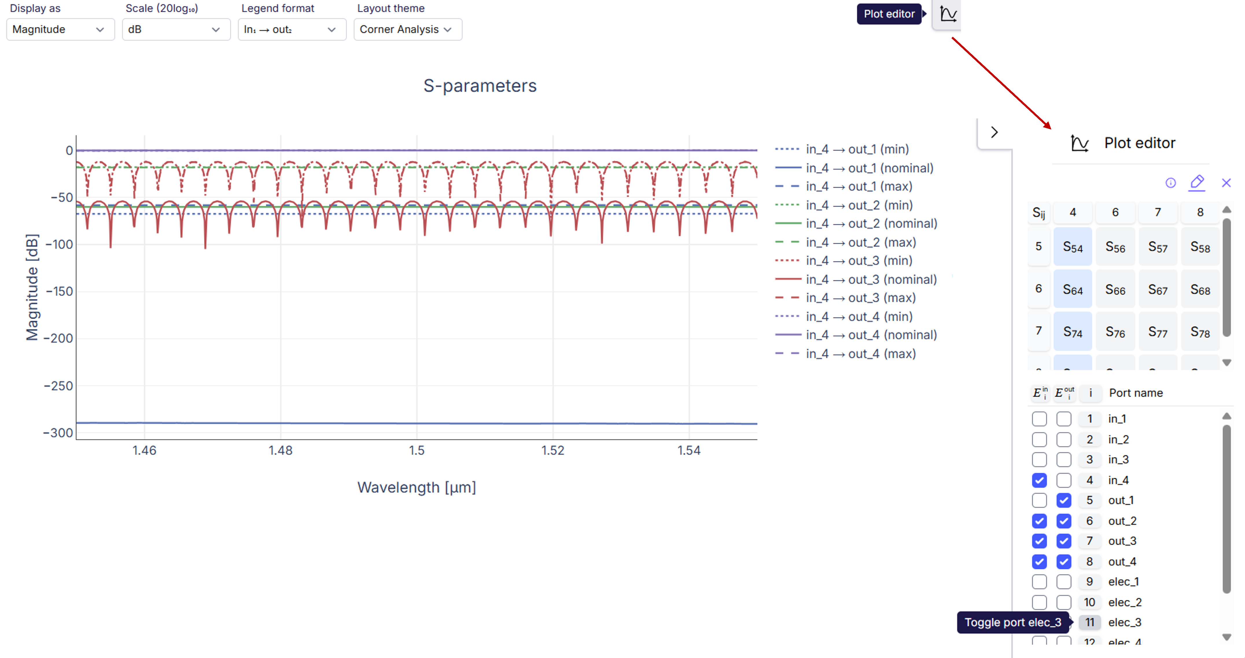
4x4 Beneš switch with selected corner analysis for input 4
In this figure, we used the Plot editor in our visualizer to open a small window to manage the s-matrix. There, we controlled the size and entries shown in the s-matrix by toggling them and selected the four entries of interest to us to plot (also selected by code before but with no need if we use the editor). As expected, if we take corners of “nominal” for all the parameters, it will correspond to the usual simulation as in the first section of this tutorial. Additionally we see the effect of the corners in dashed lines.
From Canvas, we can also open this project and run the CornerAnalysis codelet which runs ca.corner_analysis_all_combinations
and we can select which entries to observe. For completeness, the following figure plots this for input 4 as well.
This results in the following visualization of the corners:
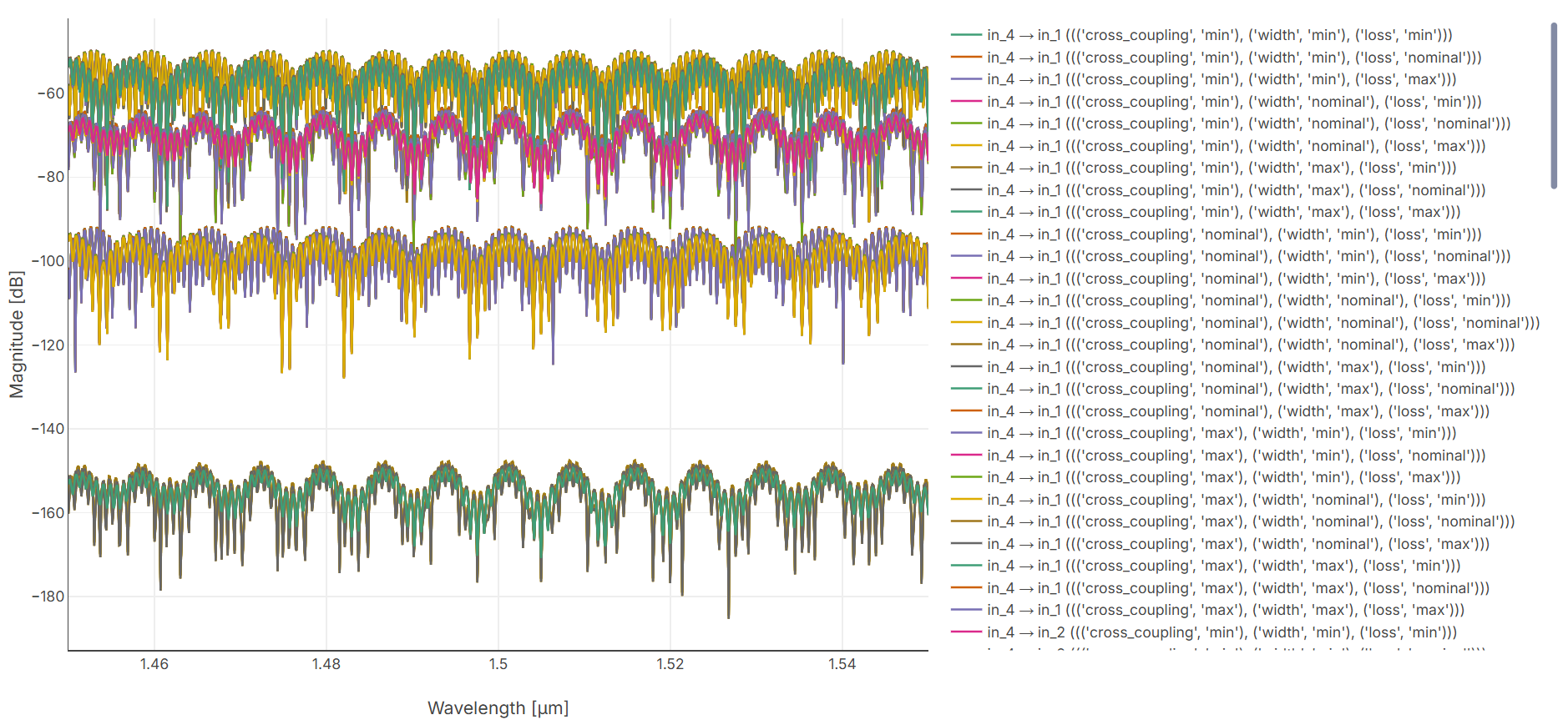
4x4 Beneš switch all corners analysis for input 4
Note
When running from Canvas, you still need to define models.py separatly and you need to provide the path to the model.yaml file to the codelet. Once that is done, you can also modify your corners directly in IPKISS Canvas.
Once the codelet is properly configured with a models.py script, Canvas allows to directly change the corners with adding new parameters, replace values and much more! A window will pop up as in next figure to allow this.
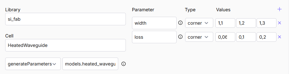
Window on IPKISS Canvas to adjust the corners in CornerAnalysis codelet
Conclusion
In this introductory tutorial for the Circuit Analyzer, we showed how to do corner analysis for the Beneš switch. Starting from a nominal simulation, we explored how to define and analyze process variations by setting up corner parameters in both the models.yaml and models.py configuration files. Finally we observed how deviations in those parameters affect the circuit’s optical response.
A next step after this tutorial can be Monte Carlo simulation. As the number of combinations grow, this gives (1) flexibility in exploring parameter distribution (for instance, following a Gaussian function) as opposed to fixed minimum, nominal and maximum and (2) to generate simulations based on these distributions to better estimate the actual circuit’s behavior. This helps predicting yield and performance variations - our ultimate goal. You can find more Circuit Analyzer examples in our academy at samples/circuit_analyzer!