Layout and simulation of a ring resonator with grating couplers

Build a small ring circuit with grating couplers. Export the layout + run a circuit simulation to verify circuit operation.

Importing the technology file

We start with importing the silicon_photonics technology, which is a basic technology shipped with IPKISS. You can replace this technology by another technology (custom-made, or from our list of supported PDKs). and the layers will automatically adjust to reflect this technology.

from si_fab import all as pdk  # noqa
from ipkiss3 import all as i3

# Import other python libraries.
import numpy as np

Creating the ring resonator

Here we use a ring resonator from the picazzo component library (the Picazzo Library is a generic component library with a wide range of photonic components).

from picazzo3.filters.ring import RingRect180DropFilter  # noqa

my_ring = RingRect180DropFilter()

# Setting the layout properties of the ring.
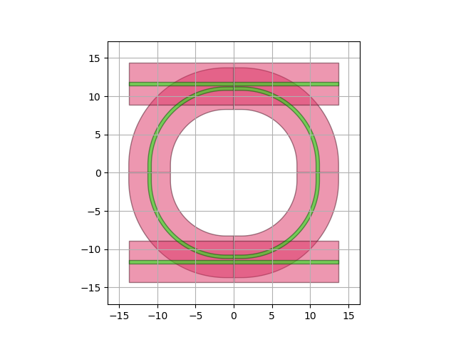
my_ring_layout = my_ring.Layout(bend_radius=10.0)  # We set the bend radius of the ring to 10.
my_ring_layout.visualize()  # We visualize the layout of the ring

Running a circuit simulation

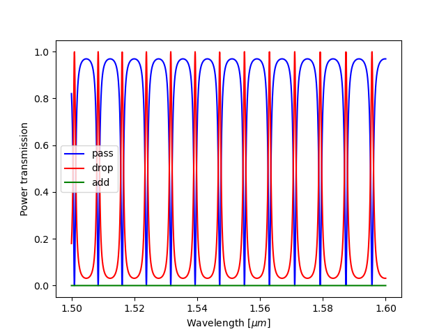
Here we set some simple model parameters for the directional coupler of the ring, and then we run a circuit simulation. Note that the waveguide lengths are automatically extracted from the layout.

cp = dict(cross_coupling1=1j * 0.3**0.5, straight_coupling1=0.7**0.5)  # The coupling from bus to ring and back

my_ring_cm = my_ring.CircuitModel(coupler_parameters=[cp, cp])  # 2 couplers

# Simulating the ring.
wavelengths = np.linspace(1.50, 1.6, 2001)
S = my_ring_cm.get_smatrix(wavelengths=wavelengths)
S.visualize(
    term_pairs=[
        ("in1", "out1"),  # pass
        ("in1", "out2"),  # drop
        ("in1", "in2"),  # add
    ]
)

Creating the grating coupler

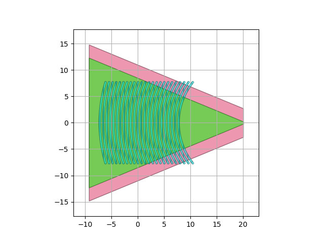
The picazzo component library also contains parametrized curved grating couplers. We will pick one to use in our circuit.

from picazzo3.fibcoup.curved import FiberCouplerCurvedGrating  # noqa

my_grating = FiberCouplerCurvedGrating()

# Setting the layout properties of the grating layout.
my_grating_layout = my_grating.Layout(n_o_lines=24, period_x=0.65, box_width=15.5)
my_grating_layout.visualize()

# Setting the properties of the circuit model and simulate.
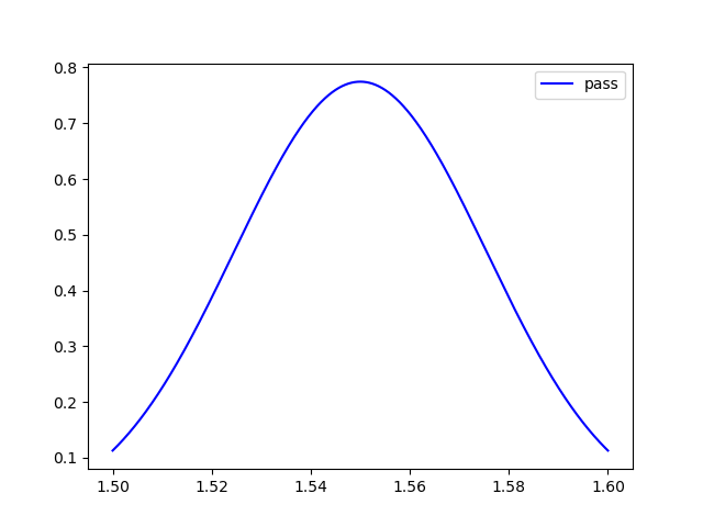
my_grating_cm = my_grating.CircuitModel(
    center_wavelength=1.55,
    bandwidth_3dB=0.06,
    peak_transmission=0.60**0.5,
    reflection=0.05**0.5,
)

S = my_grating_cm.get_smatrix(wavelengths=wavelengths)
S.visualize(
    term_pairs=[
        ("vertical_in", "out"),  # pass
    ]
)

• 
• 

Creating a small circuit with the ring and grating coupler

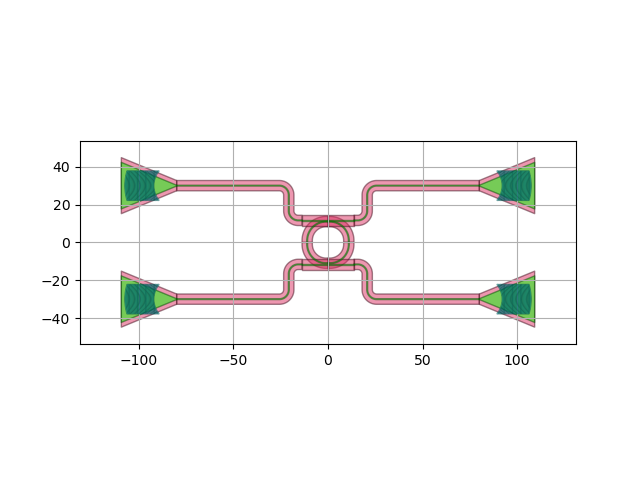
Next, we can use some high-level routing functionality from IPKISS to place the grating couplers and the ring, and route waveguides between them. This is done using ipkiss3.all.Circuit.

distance_x = 100.0
distance_y = 30.0

my_circuit = i3.Circuit(
    insts={
        "in_grating": my_grating,
        "pass_grating": my_grating,
        "add_grating": my_grating,
        "drop_grating": my_grating,
        "ring": my_ring,
    },
    specs=[
        i3.Place("ring", (0, 0)),
        i3.Place("in_grating", (-distance_x, -distance_y)),
        i3.Place("pass_grating", (distance_x, -distance_y), angle=180),
        i3.Place("add_grating", (distance_x, distance_y), angle=180),
        i3.Place("drop_grating", (-distance_x, distance_y)),
        i3.ConnectManhattan(
            [
                ("in_grating:out", "ring:in1"),
                ("pass_grating:out", "ring:out1"),
                ("add_grating:out", "ring:in2"),
                ("drop_grating:out", "ring:out2"),
            ]
        ),
    ],
    exposed_ports={
        "add_grating:vertical_in": "add",
        "drop_grating:vertical_in": "drop",
        "in_grating:vertical_in": "in",
        "pass_grating:vertical_in": "pass",
    },
)

my_circuit_layout = my_circuit.Layout()

my_circuit_layout.visualize()

# Simulate the circuit.
my_circuit_cm = my_circuit.CircuitModel()
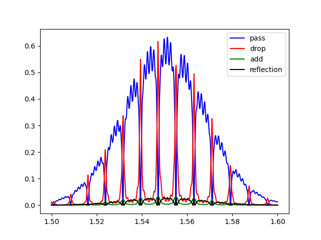
S = my_circuit_cm.get_smatrix(wavelengths=wavelengths)
S.visualize(
    term_pairs=[
        ("in", "pass"),  # pass
        ("in", "drop"),  # drop
        ("in", "add"),  # add
        ("in", "in"),  # reflection
    ]
)

• 
• 

You can clearly see the following features in this response:

• the grating response: the grating was designed for 1550 nm, and has a gaussian-like profile,

• the ring resonances

• there are some ripples on the circuit response, this is due to reflections on the grating couplers.

Caphe is a bidirectional-aware circuit solver (each optical port has a forward and backward propagating wave), and this is how we can capture these important parasitic effects.