Note
Go to the end to download the full example code
SpectrumAnalyzer: how to use it to analyze the results from simulation or measurement
In this example, we demonstrate how to use i3.SpectrumAnalyzer
to visualize and analyze the simulation and measurement data through a real case
(MUX4),
obtain some key performance indices, and compare the differences between simulation and measurement results.
Note
Please download the Touchstone mux4_measurement_smatrix.s8p and CSV mux4_measurement_data.csv
files before running this example.
Analyze simulation results
We copy the ‘MUX4’ class from the CWDM transmitter application example. Then we use it to generate a 4-way demultiplexer and get its simulation results.
from si_fab import all as pdk  # noqa: F401
from ipkiss3 import all as i3
import pteam_library_si_fab.all as pt_lib
import numpy as np
import json
import os
import matplotlib.gridspec as gridspec
import matplotlib.pyplot as plt


class Mux4(i3.Circuit):
    spacing_x = i3.PositiveNumberProperty(default=100.0, doc="Port-to-port spacing between the MUXs in the x-direction")
    spacing_y = i3.PositiveNumberProperty(default=150.0, doc="Port-to-port spacing between the MUXs in the y-direction")
    bend_radius = i3.PositiveNumberProperty(default=5.0, doc="Bend radius")
    fsr = i3.PositiveNumberProperty(default=0.02, doc="Free spectral range of the MUX4")
    center_wavelength = i3.PositiveNumberProperty(default=1.55, doc="Center wavelength")
    stage_1 = i3.ChildCellProperty(doc="MUX2 for the first stage")
    stage_2_up = i3.ChildCellProperty(doc="MUX2 for the second stage (up)")
    stage_2_down = i3.ChildCellProperty(doc="MUX2 for the second stage (down)")

    def _default_stage_1(self):
        return pt_lib.Mux2(
            center_wavelength=self.center_wavelength,
            fsr=self.fsr / 2.0,
            name=self.name + "_stage1",
        )

    def _default_stage_2_up(self):
        return pt_lib.Mux2(
            center_wavelength=self.center_wavelength + self.fsr / 4,
            fsr=self.fsr,
            name=self.name + "_stage2_up",
        )

    def _default_stage_2_down(self):
        return pt_lib.Mux2(
            center_wavelength=self.center_wavelength,
            fsr=self.fsr,
            name=self.name + "_stage2_down",
        )

    def _default_specs(self):
        specs = [
            i3.Inst("mux_0_0", self.stage_1),
            i3.Inst("mux_1_0", self.stage_2_down),
            i3.Inst("mux_1_1", self.stage_2_up),
            i3.Place("mux_0_0", (0, 0)),
            i3.Place("mux_1_0:in1", (self.spacing_x, -self.spacing_y / 2), relative_to="mux_0_0:out1"),
            i3.Place("mux_1_1:in1", (self.spacing_x, +self.spacing_y / 2), relative_to="mux_0_0:out2"),
        ]

        specs += [
            i3.ConnectManhattan(
                [
                    ("mux_0_0:out1", "mux_1_0:in1"),
                    ("mux_0_0:out2", "mux_1_1:in1"),
                ],
                bend_radius=self.bend_radius,
            )
        ]
        return specs

    def _default_exposed_ports(self):
        return {
            "mux_0_0:in1": "in1",
            "mux_0_0:in2": "in2",
            "mux_1_0:in2": "in3",
            "mux_1_1:in2": "in4",
            "mux_1_0:out1": "out1",
            "mux_1_0:out2": "out2",
            "mux_1_1:out1": "out3",
            "mux_1_1:out2": "out4",
        }
After defining the Mux4 circuit, you can generate its layout and export it to a GDSII file Set the simulation wavelength range and obtain the S-matrix within that wavelength range by calling the Circuit Model. And then save the generated S matrix as a Touchstone file.
cell = Mux4(
    name="MUX4",
    fsr=0.048,
    center_wavelength=1.55,
    spacing_x=50,
    spacing_y=80,
)
cell_lv = cell.Layout()
cell_lv.visualize(show=False, annotate=True)
cell_lv.write_gdsii("mux4.gds")

wavelengths = np.linspace(1.5, 1.6, 501)
cell_cm = cell.CircuitModel()
S_total = cell_cm.get_smatrix(wavelengths=wavelengths)
smatrix_path = os.path.join(f"mux4_simulation_smatrix.s{S_total.data.shape[0]}p")
S_total.to_touchstone(smatrix_path)
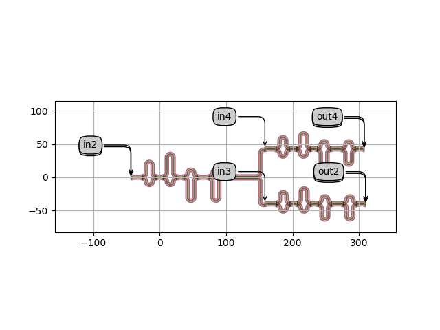
Now, let’s use the SpectrumAnalyzer to analyze and visualize the simulation results.
Specify input and output ports: Begin by defining the input and output ports for the analysis.
Select power units: Whether to analyze the smatrix power in decibel (True) or linear scale (False).
Set the peak detection method and threshold: Choose the peak detection method and adjust the threshold to ensure that only peaks with power exceeding this value are detected.
Set the bandpass parameter: Treat spectra as bandpass (True), bandstop (False) or automatic (None).
output_ports = ["out1", "out2", "out3", "out4"]

simulation = i3.SpectrumAnalyzer(
    S_total,
    input_port_mode="in1",
    output_port_modes=output_ports,
    dB=True,
    peak_method="spline",
    peak_threshold=-5,
    bandpass=True,
)
simulation.visualize(show=True, title="mux4 simulation Spectrum")
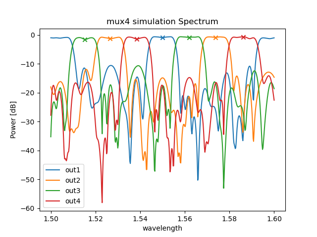
The SpectrumAnalyzer enables the extraction of key performance indices, such as insertion loss, crosstalk, and 3dB passband width. Here’s how to calculate these metrics:
channel_width = 0.0001  # Specify the channel bandwidth.
peaks = simulation.peaks()  # Search for the peaks of the channel and return the wavelengths and powers of the peaks.
bands = simulation.width_passbands(
    channel_width
)  # Search for the passband range of each channel according to the specified bandwidth.
min_insertion_loss = simulation.min_insertion_losses(
    bands=bands
)  # The minimum insertion loss within the passband range of each channel.
max_insertion_loss = simulation.max_insertion_losses(
    bands=bands
)  # The maximum insertion loss within the passband range of each channel.
crosstalk_near = simulation.near_crosstalk_matrix(
    bands=bands
)  # The adjacent crosstalk within the passband range of each channel.
crosstalk_far = simulation.far_crosstalk_matrix(
    bands=bands
)  # The non-Adjacent crosstalk within the passband range of each channel.
passbands_3dB = simulation.cutoff_passbands(
    cutoff=-3.0
)  # The bandwidth range where the maximum peak value of each channel decreases by 3dB
Finally, the analysis results are saved in a JSON report for easy review
report = dict()
for cnt, port in enumerate(output_ports):
    channel_report = {
        "peak": peaks[port],
        "band": bands[port],
        "passbands_3dB": passbands_3dB[port],
        "min_insertion_loss": min_insertion_loss[port],
        "max_insertion_loss": max_insertion_loss[port],
        "crosstalk_near": crosstalk_near[port],
        "cross_talk_far": crosstalk_far[port],
    }
    report[port] = channel_report


def serialize_ndarray(obj):
    return obj.tolist() if isinstance(obj, np.ndarray) else obj


report_path = os.path.join("mux4_simulation_report.json")
with open(report_path, "w") as f:
    json.dump(report, f, sort_keys=True, default=serialize_ndarray, indent=4)
print(f"{report_path} written")
print(json.dumps(report, indent=4, default=serialize_ndarray))
mux4_simulation_report.json written
{
    "out1": {
        "peak": [
            [
                1.55,
                -0.9444522032753643
            ]
        ],
        "band": [
            [
                1.54995,
                1.5500500000000001
            ]
        ],
        "passbands_3dB": [
            [
                1.5442,
                1.5558
            ]
        ],
        "min_insertion_loss": [
            -0.938708756221252
        ],
        "max_insertion_loss": [
            -0.9444522032753643
        ],
        "crosstalk_near": {
            "out3": [
                -16.72919405448907
            ],
            "out4": [
                -16.544869242949993
            ]
        },
        "cross_talk_far": {
            "out2": [
                -13.912602623734006
            ]
        }
    },
    "out2": {
        "peak": [
            [
                1.5268,
                -1.288571780354546
            ],
            [
                1.5738,
                -0.8407794458925938
            ]
        ],
        "band": [
            [
                1.5267499999999998,
                1.52685
            ],
            [
                1.57375,
                1.5738500000000002
            ]
        ],
        "passbands_3dB": [
            [
                1.5208,
                1.5328
            ],
            [
                1.568,
                1.5796000000000001
            ]
        ],
        "min_insertion_loss": [
            -1.288571780354546,
            -0.825450929856366
        ],
        "max_insertion_loss": [
            -1.2965115011635253,
            -0.8407794458925938
        ],
        "crosstalk_near": {
            "out3": [
                -15.919720849533642,
                -16.11565923463627
            ],
            "out4": [
                -19.051033042946724,
                -15.708270671629684
            ]
        },
        "cross_talk_far": {
            "out1": [
                -9.288233009189401,
                -25.466039318370054
            ]
        }
    },
    "out3": {
        "peak": [
            [
                1.5156,
                -1.5284760239235031
            ],
            [
                1.562,
                -0.8336931821991745
            ]
        ],
        "band": [
            [
                1.51555,
                1.5156500000000002
            ],
            [
                1.56195,
                1.5620500000000002
            ]
        ],
        "passbands_3dB": [
            [
                1.51,
                1.521
            ],
            [
                1.5558,
                1.568
            ]
        ],
        "min_insertion_loss": [
            -1.5284760239235031,
            -0.8216274424252734
        ],
        "max_insertion_loss": [
            -1.5394856512859603,
            -0.8336931821991745
        ],
        "crosstalk_near": {
            "out1": [
                -10.085442288151427,
                -21.64968474015515
            ],
            "out2": [
                -10.708156990288714,
                -20.558351973695665
            ]
        },
        "cross_talk_far": {
            "out4": [
                -15.829928448870536,
                -13.918581592346376
            ]
        }
    },
    "out4": {
        "peak": [
            [
                1.5384,
                -1.3932023495798085
            ],
            [
                1.5862,
                -0.6647203554820341
            ]
        ],
        "band": [
            [
                1.5383499999999999,
                1.53845
            ],
            [
                1.58615,
                1.5862500000000002
            ]
        ],
        "passbands_3dB": [
            [
                1.5326,
                1.5442
            ],
            [
                1.5798,
                1.5924
            ]
        ],
        "min_insertion_loss": [
            -1.3932023495798085,
            -0.6647203554820341
        ],
        "max_insertion_loss": [
            -1.3975490554979162,
            -0.6717425930462557
        ],
        "crosstalk_near": {
            "out1": [
                -13.165132093643603,
                -27.911782067227854
            ],
            "out2": [
                -14.336175620432961,
                -26.892259964319262
            ]
        },
        "cross_talk_far": {
            "out3": [
                -9.418079850460291,
                -27.094982971626198
            ]
        }
    }
}
Analyze measurements result and compare to simulation in Touchstone file
If we have obtained the measured result, how should we process it?
Using the same method i3.SpectrumAnalyzer,
we can also handle measured Touchstone files.
Import the Touchstone file: Use the
SMatrix1DSweepto convert the Touchstone file into an S-matrix.Process the S-matrix: Use the
i3.SpectrumAnalyzerto process the S-matrix and obtain the transmission spectrum and specified performance indices.
def create_spectrum_analyzer(file_path):
    # Load the S-parameters from the Touchstone file
    smatrix = i3.device_sim.SMatrix1DSweep.from_touchstone(file_path, unit="um")

    # Set up the SpectrumAnalyzer with specified options
    return i3.SpectrumAnalyzer(
        smatrix=smatrix,
        input_port_mode="in1",
        output_port_modes=output_ports,
        peak_method="spline",  # Peak detection method
        peak_threshold=-5,  # Threshold for peak detection
        dB=True,
        bandpass=True,
    )


touchstone_file_paths = [r"mux4_measurement_smatrix.s8p", r"mux4_simulation_smatrix.s8p"]
# Create SpectrumAnalyzer objects for both measurement and simulation data
measurement = create_spectrum_analyzer(touchstone_file_paths[0])
simulation = create_spectrum_analyzer(touchstone_file_paths[1])
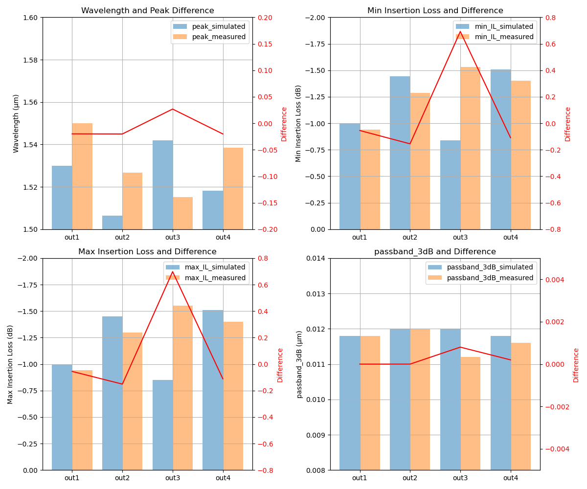
To visually illustrate the actual performance of the device, we will plot the measured result and include a comparison chart with the simulated result.
def plot_spectrum(ax, channels, title, linestyle, colors):
    # Function to plot spectra for comparison
    for i, (name, spectrum) in enumerate(channels.items()):
        wav = spectrum.x
        y = spectrum.power
        color = colors[i % len(colors)]
        ax.plot(wav, y, label=name, linestyle=linestyle, color=color)
    ax.set_title(title)
    ax.legend()


fig = plt.figure(figsize=(10, 10))
gs = gridspec.GridSpec(2, 2)

# Create subplots for the simulation and measurement spectra
ax1 = fig.add_subplot(gs[0, 0])
ax2 = fig.add_subplot(gs[0, 1])
ax3 = fig.add_subplot(gs[1, :])

# Plot the simulation and measurement spectra
colors = ["blue", "orange", "green", "red"]
plot_spectrum(ax1, simulation.channels, "simulation", linestyle="--", colors=colors)
plot_spectrum(ax2, measurement.channels, "measurement", linestyle="-", colors=colors)
plot_spectrum(ax3, simulation.channels, "mix", linestyle="--", colors=colors)
plot_spectrum(ax3, measurement.channels, "mix", linestyle="-", colors=colors)
plt.tight_layout()
plt.show()
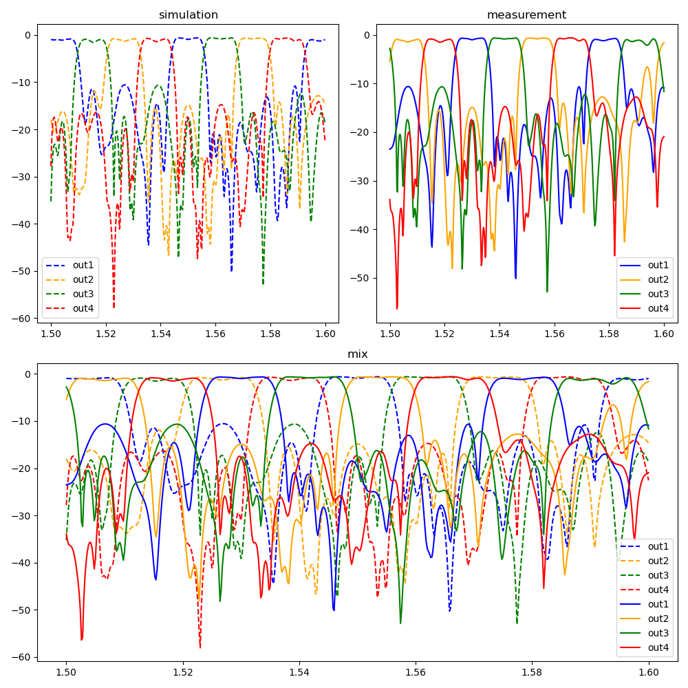
Simultaneously, to quantitatively assess the actual performance of the device, we calculated performance indices such as the central wavelength, insertion loss, and 3-dB bandwidth. Additionally, we compared these metrics with the simulation results.
def calculate_performance_indices(content, output_ports, channel_width=0.0001):
    """
    Calculate performance indices (like peak wavelength, insertion loss, crosstalk, etc.)
    for each output port.

    Parameters:
    - content: SpectrumAnalyzer object (measurement or simulation).
    - output_ports: List of output ports to analyze.
    - channel_width: Passband width for analysis.

    Returns:
    - A dictionary containing performance indices for each port.
    """
    # Extract peak, bandwidth, insertion loss, and crosstalk values for the given ports
    peaks = content.peaks()
    bands = content.width_passbands(channel_width)
    min_insertion_loss = content.min_insertion_losses(bands=bands)
    max_insertion_loss = content.max_insertion_losses(bands=bands)
    crosstalk_near = content.near_crosstalk_matrix(bands=bands)
    crosstalk_far = content.far_crosstalk_matrix(bands=bands)
    passbands_3dB = content.cutoff_passbands(cutoff=-3.0)

    # Prepare a dictionary with performance indices for each output port
    performance_indices = {
        port: {
            "peak": peaks[port],
            "band": bands[port],
            "passbands_3dB": passbands_3dB[port],
            "min_insertion_loss": min_insertion_loss[port],
            "max_insertion_loss": max_insertion_loss[port],
            "crosstalk_near": crosstalk_near[port],
            "crosstalk_far": crosstalk_far[port],
        }
        for port in output_ports
    }

    return performance_indices


# Calculate performance indices for simulation and measurement
performance_data_sim = calculate_performance_indices(content=measurement, output_ports=output_ports)
performance_data_meas = calculate_performance_indices(content=simulation, output_ports=output_ports)


def generate_comparison_report(simulation, Measurement, output_ports):
    comparison_report = {}

    first_channel_simulation = simulation.peaks()["out1"]
    first_channel_measurement = Measurement.peaks()["out1"]

    # Calculate the difference in wavelength and insertion loss between simulation and measurement
    diffs = np.abs(first_channel_simulation["wavelength"][:, np.newaxis] - first_channel_measurement["wavelength"])
    min_index_2d = np.unravel_index(np.argmin(diffs), diffs.shape)
    sim, meas = min_index_2d

    # Generate a report comparing the simulated and measured values for each output port
    for port in output_ports:
        comparison_report[port] = {
            "peak_simulated": performance_data_sim[port]["peak"]["wavelength"][sim],
            "peak_measured": performance_data_meas[port]["peak"]["wavelength"][meas],
            "peak_Difference": performance_data_sim[port]["peak"]["wavelength"][sim]
            - performance_data_meas[port]["peak"]["wavelength"][meas],
            "min_IL_simulated": performance_data_sim[port]["min_insertion_loss"][sim],
            "min_IL_measured": performance_data_meas[port]["min_insertion_loss"][meas],
            "min_IL_Difference": performance_data_sim[port]["min_insertion_loss"][sim]
            - performance_data_meas[port]["min_insertion_loss"][meas],
            "max_IL_simulated": performance_data_sim[port]["max_insertion_loss"][sim],
            "max_IL_measured": performance_data_meas[port]["max_insertion_loss"][meas],
            "max_IL_Difference": performance_data_sim[port]["max_insertion_loss"][sim]
            - performance_data_meas[port]["max_insertion_loss"][meas],
            "passband_3dB_simulated": performance_data_sim[port]["passbands_3dB"][sim][1]
            - performance_data_sim[port]["passbands_3dB"][sim][0],
            "passband_3dB_measured": performance_data_meas[port]["passbands_3dB"][meas][1]
            - performance_data_meas[port]["passbands_3dB"][meas][0],
            "passband_3dB_Difference": performance_data_sim[port]["passbands_3dB"][sim][1]
            - performance_data_sim[port]["passbands_3dB"][sim][0]
            - performance_data_meas[port]["passbands_3dB"][meas][1]
            + performance_data_meas[port]["passbands_3dB"][meas][0],
        }

    return comparison_report


def plot_comparison_report(comparison_report, output_ports):
    data = {
        "peak_simulated": [],
        "peak_measured": [],
        "peak_Difference": [],
        "min_IL_simulated": [],
        "min_IL_measured": [],
        "min_IL_Difference": [],
        "max_IL_simulated": [],
        "max_IL_measured": [],
        "max_IL_Difference": [],
        "passband_3dB_simulated": [],
        "passband_3dB_measured": [],
        "passband_3dB_Difference": [],
    }

    for port in output_ports:
        for key in data:
            data[key].append(comparison_report[port][key])

    X_axis = np.arange(len(output_ports))
    fig, axes = plt.subplots(2, 2, figsize=(12, 10))

    def plot_bars(ax, sim, meas, diff, ylabel, title, ylim_1, ylim_2):
        ax.bar(X_axis - 0.2, data[sim], width=0.4, label=sim, alpha=0.5)
        ax.bar(X_axis + 0.2, data[meas], width=0.4, label=meas, alpha=0.5)
        ax.set_xticks(X_axis)
        ax.set_xticklabels(output_ports)
        ax.set_ylabel(ylabel)
        ax.legend()
        ax.grid()
        ax.set_title(title)
        ax.set_ylim(ylim_1)
        ax2 = ax.twinx()
        ax2.plot(output_ports, data[diff], color="red", label=diff)
        ax2.set_ylabel("Difference", color="red")
        ax2.tick_params(axis="y", labelcolor="red")
        ax2.set_ylim(ylim_2)

    plot_bars(
        axes[0, 0],
        "peak_simulated",
        "peak_measured",
        "peak_Difference",
        "Wavelength (μm)",
        "Wavelength and Peak Difference",
        (1.5, 1.6),
        (-0.2, 0.2),
    )
    plot_bars(
        axes[0, 1],
        "min_IL_simulated",
        "min_IL_measured",
        "min_IL_Difference",
        "Min Insertion Loss (dB)",
        "Min Insertion Loss and Difference",
        (0, -2),
        (-0.8, 0.8),
    )
    plot_bars(
        axes[1, 0],
        "max_IL_simulated",
        "max_IL_measured",
        "max_IL_Difference",
        "Max Insertion Loss (dB)",
        "Max Insertion Loss and Difference",
        (0, -2),
        (-0.8, 0.8),
    )
    plot_bars(
        axes[1, 1],
        "passband_3dB_simulated",
        "passband_3dB_measured",
        "passband_3dB_Difference",
        "passband_3dB (μm)",
        "passband_3dB and Difference",
        (0.008, 0.014),
        (-0.005, 0.005),
    )

    fig.tight_layout()
    plt.show()


# Export the comparison report and visualize it.
comparison_report = generate_comparison_report(simulation, measurement, output_ports)
plot_comparison_report(comparison_report, output_ports)

# Analyze measurements result in CSV file
# ---------------------------------------
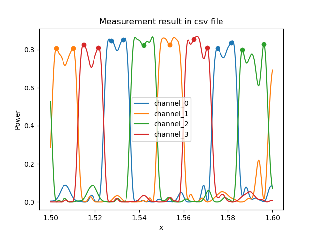
If your measurement result is not a Touchstone file but a CSV file with wavelength-dependent transmission data,
you can use another function i3.Spectrum
according to the following steps.
First, read the CSV file to extract wavelength and transmission data.
Pass the wavelength and power data to the function, assigning wavelength to x and transmission to power.
Similarly, you can use
i3.Spectrumto obtain performance indices such as peak value and insertion loss.
# Read csv file.
data = np.loadtxt("mux4_measurement_data.csv", delimiter=",", skiprows=1)

# Extract the first column as lambda.
lambda_values = data[:, 0]

# Extract the subsequent output columns as transmission
transmissions = [data[:, i] for i in range(1, data.shape[1])]
fig = plt.figure()
# Use i3.Spectrum to visualize the transmission spectrum and analyze performance indices.
for idx, transmission in enumerate(transmissions):
    spectrum = i3.Spectrum(
        x=lambda_values,
        power=transmissions[idx],
        dB=False,
        peak_method="spline",
        bandpass=True,
        peak_threshold=0.8,
    )
    spectrum.visualize(show=False, label=f"channel_{idx}", figure=fig)

    peaks = spectrum.find_peaks(method="spline", threshold=0.8, bandpass=True)
    channel_width = 0.0001
    bands = spectrum.width_passbands(width=channel_width)
    bandwidth_3db = spectrum.cutoff_passbands(cutoff=-3)
    min_insertion_loss = spectrum.min_insertion_losses(bands=bands)
    max_insertion_loss = spectrum.max_insertion_losses(bands=bands)

plt.title("Measurement result in csv file")
plt.legend()
plt.show()
