Note
Go to the end to download the full example code
Analyzing Kerr nonlinearity in optical ring resonators
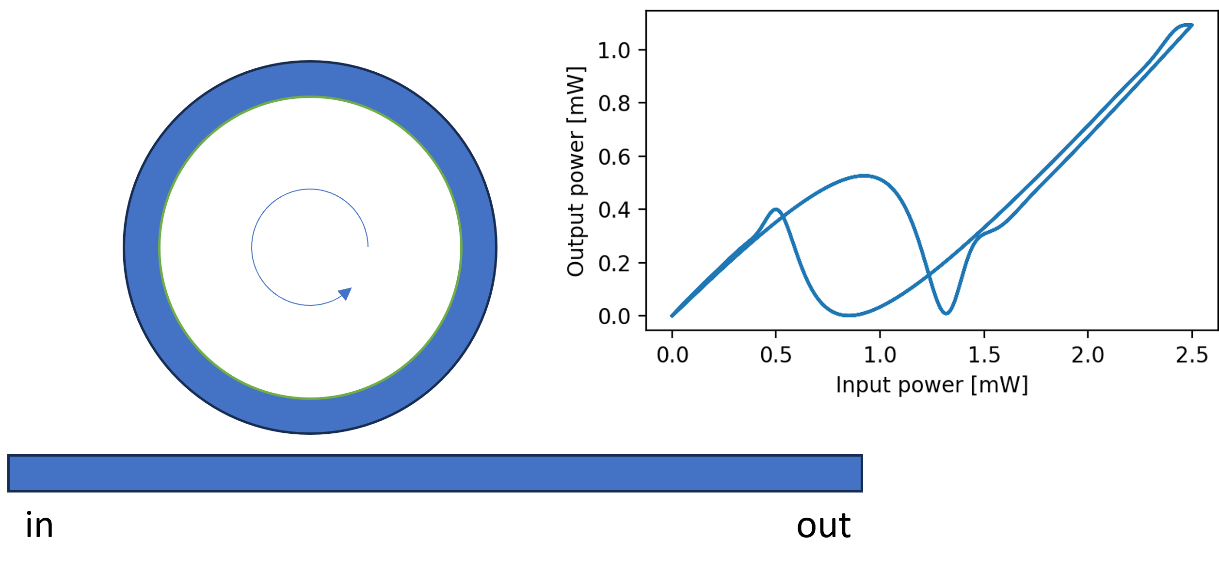
This sample illustrates how to build a nonlinear model (Kerr nonlinearity) for an optical resonator and run a time-domain analysis to observe bistability.

The models are based on “Self-pulsing and chaos in short chains of coupled nonlinear microcavities”. (see references below).
import ipkiss3.all as i3
import numpy as np
from scipy.constants import speed_of_light as c
import matplotlib.pyplot as plt
Constructing the model
To write a compact model in IPKISS we need to describe the time and frequency dependent behavior. More explanation on how to build models can be found in Creating a First Circuit Simulation. For this model, we make a few assumptions:
We only describe the time-dependent behavior.
We only consider 1 mode (counterclockwise).
We only describe the Kerr nonlinearity.
All model parameters are normalized, a conversion is needed to translate to SI units.
#   This could be extended to also include temperature, two-photon absorption etc, ...


class RingModel(i3.CompactModel):
    parameters = [
        "wavelength_res",  # resonance wavelength
        "phi",  # phase shift in transmission
        "P0",  # characteristic nonlinear power
        "tau",  # photon lifetime
    ]

    states = ["ring_energy_ccw"]  # counterclockwise mode of the ring

    terms = [
        i3.OpticalTerm(name="in", n_modes=1),
        i3.OpticalTerm(name="out", n_modes=1),
        i3.OpticalTerm(name="energy_probe", n_modes=1),  # used for debugging the energy in the ring
        i3.OpticalTerm(
            name="detuning_probe", n_modes=1
        ),  # used for debugging the current detuning (including nonlinear contributions)
    ]

    def calculate_smatrix(parameters, env, S):
        raise NotImplementedError("RingModel contains no frequency domain model.")

    def calculate_signals(parameters, env, output_signals, y, t, input_signals):
        # d: coupling coefficient
        d = 1j * np.exp(1j * parameters.phi / 2) / np.sqrt(parameters.tau)

        output_signals["out"] = np.exp(1j * parameters.phi) * input_signals["in"] + d * y["ring_energy_ccw"]
        output_signals["in"] = np.exp(1j * parameters.phi) * input_signals["out"] + d * y["ring_energy_ccw"]

        # This one is purely for debugging: for measuring the energy in the ring.
        output_signals["energy_probe"] = y["ring_energy_ccw"]
        # Also for debugging: the final detuning.
        omega = 2 * np.pi * c / env.wavelength
        omega_0 = 2 * np.pi * c / parameters.wavelength_res

        delta_omega = -(np.abs(y["ring_energy_ccw"]) ** 2) / (parameters.P0 * parameters.tau**2)
        output_signals["detuning_probe"] = parameters.tau * (omega_0 - omega + delta_omega)

    def calculate_dydt(parameters, env, dydt, y, t, input_signals):
        # Here we describe how the state 'y' (energy in the ring) changes with time.
        delta_omega = -(np.abs(y["ring_energy_ccw"]) ** 2) / (parameters.P0 * parameters.tau**2)
        d = 1j * np.exp(1j * parameters.phi / 2) / np.sqrt(parameters.tau)
        omega = 2 * np.pi * c / env.wavelength
        omega_0 = 2 * np.pi * c / parameters.wavelength_res
        t1 = (1j * (omega_0 - omega + delta_omega) - 1 / parameters.tau) * y["ring_energy_ccw"]
        t2 = d * (input_signals["in"])  # Only counterclockwise, signal comes from the input
        dydt["ring_energy_ccw"] = t1 + t2


# Define a PCell for the ring which only includes the netlist and model. No layout is required to run simulation.
class Ring(i3.PCell):
    class Netlist(i3.NetlistView):
        def _generate_terms(self, terms):
            terms += i3.OpticalTerm(name="in")
            terms += i3.OpticalTerm(name="out")
            terms += i3.OpticalTerm(name="energy_probe")
            terms += i3.OpticalTerm(name="detuning_probe")
            return terms

    class CircuitModel(i3.CircuitModelView):
        wavelength_res = i3.PositiveNumberProperty(doc="Resonance wavelength [um]", default=1.55e-6)
        phi = i3.NumberProperty(doc="Phase shift in transmission", default=0.0)
        P0 = i3.PositiveNumberProperty(doc="characteristic nonlinear power [W/rad]", default=1.0e-3)
        tau = i3.PositiveNumberProperty(doc="Photon lifetime [s]", default=1.0e-9)

        def _generate_model(self):
            return RingModel(wavelength_res=self.wavelength_res, phi=self.phi, P0=self.P0, tau=self.tau)
Setting up the testbench
Next we define simulation parameters and set up a testbench:
tau = 1.5e-9
P0 = 0.5e-3
input_power = 10e-3
phi = 0.0
period = 100 * tau

detuning_ghz = -200 * 1e6
wavelength_res = 1.55e-6
wavelength_sim = c / (detuning_ghz + c / wavelength_res)

omega_sim = 2 * np.pi * c / wavelength_sim
omega_0 = 2 * np.pi * c / wavelength_res

detuning = tau * (omega_0 - omega_sim)


def sawtooth_function(period, amplitude):
    def _sawtooth(t):
        where = (t % period) / period
        if where < 0.5:
            return where * amplitude
        else:
            return (1 - where) * amplitude

    return _sawtooth


ring = Ring()
ring.CircuitModel(wavelength_res=wavelength_res, tau=tau, P0=P0)

sawtooth = sawtooth_function(period, input_power**0.5)  # Optical excitation applied to the ring.

circuit = i3.ConnectComponents(
    child_cells={
        "input_signal": i3.FunctionExcitation(
            port_domain=i3.OpticalDomain,
            excitation_function=sawtooth,
        ),
        "output_signal": i3.Probe(port_domain=i3.OpticalDomain),
        "ring_energy": i3.Probe(port_domain=i3.OpticalDomain),
        "delta_omega": i3.Probe(port_domain=i3.OpticalDomain),
        "ring": ring,
    },
    links=[
        ("input_signal:out", "ring:in"),
        ("ring:out", "output_signal:in"),
        ("ring:energy_probe", "ring_energy:in"),
        ("ring:detuning_probe", "delta_omega:in"),
    ],
)
Running the simulations
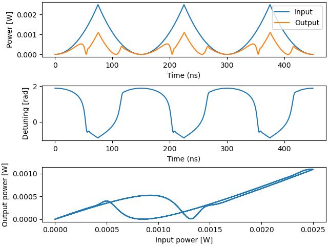
Finally we run the simulations and plot the results. The first plot shows the input and output signal as function of time. The second plot shows the detuning, which is a measure of how off-resonance the ring is (0 = on resonance). The third plot shows the output as function of the input, where bistability can be observed.
cm = circuit.CircuitModel()

center_wavelength = 2 * np.pi / omega_sim

time_response = cm.get_time_response(
    t0=0,
    dt=0.1 * tau,
    t1=300 * tau,
    center_wavelength=2 * np.pi * c / omega_sim,
)

fig, (ax1, ax2, ax3) = plt.subplots(3, 1, layout="constrained")

ax1.plot(time_response.timesteps * 1e9, np.abs(time_response["input_signal"]) ** 2, label="Input")
ax1.plot(time_response.timesteps * 1e9, np.abs(time_response["output_signal"]) ** 2, label="Output")
ax1.set_xlabel("Time (ns)")
ax1.set_ylabel("Power [W]")
ax1.legend()

ax2.plot(time_response.timesteps * 1e9, np.real(time_response["delta_omega"]), label="Detuning")
ax2.set_xlabel("Time (ns)")
ax2.set_ylabel("Detuning [rad]")

ax3.plot(np.abs(time_response["input_signal"]) ** 2, np.abs(time_response["output_signal"]) ** 2)
ax3.set_xlabel("Input power [W]")
ax3.set_ylabel("Output power [W]")
plt.show()

Conclusion
This is a very small example illustrating how to build and simulate a ring resonator model with a Kerr (chi3) nonlinearity. This model is deliberately kept very simple, but can be extended to include both clockwise and counterclockwise mode, coupling between the modes (due to the surface roughness in the ring), as well as other effects such as two photon absorption, temperature, and so on.
We only investigated a single device in this example, but with IPKISS you can now build larger circuits that include other types of devices and models (photodetectors, modulators, passive devices).
In “Nanophotonic Reservoir Computing Using Photonic Crystal Cavities” (see references) an extensive study is made where large networks of coupled resonators are combined in various topologies, and the nonlinear dynamic behavior is studied to observe regions of self-pulsation and chaos. It also studies how systems can be used for reservoir computing and to generate arbitrary waveform patterns.
References
Equations and analysis:
“Analytical study of optical bistability in silicon ring resonators” January 1, 2010 / Vol. 35, No. 1 / OPTICS LETTERS
“Self-pulsing and chaos in short chains of coupled nonlinear microcavities” PHYSICAL REVIEW A 80, 033805 (2009) (http://photonics.intec.ugent.be/download/pub_2427.pdf)
“Nanophotonic Reservoir Computing Using Photonic Crystal Cavities”, chapter 3.2 “Simulation of photonic crystal cavities” (http://photonics.intec.ugent.be/download/phd_190.pdf)