Note
Go to the end to download the full example code
Defining a compact model for thermal MZI
In this example, we first define a temperature-dependent compact model of a waveguide. Then, we employ this custom model for the waveguides of a Mach-Zehnder interferometer to perform a temperature-dependent simulation.
Getting started
We start by importing the technology and other necessary modules:
import matplotlib.pyplot as plt
from si_fab import all as pdk
import ipkiss3.all as i3
import numpy as np
The temperature-dependent waveguide model
This takes into account the effect of temperature, which is taken from env, just like the wavelength.
The behavior in frequency-domain is fully described by the S-matrix, which we compute in calculate_smatrix.
class ThermalWGCompactModel(i3.CompactModel):
    """Single mode waveguide model with thermal effects.

    Parameters
    ----------
    n_eff: float
       Effective index at center_wavelength.
    n_g: float
       Group index at center_wavelength.
    center_wavelength: float (m)
        Center wavelength (in meter) of the model around which n_eff and loss are defined.
    loss: float (dB/m)
        Waveguide loss in dB/m.
    length: float (m)
       Total length of the waveguide in meter.
    reference_temperature (K)
        At temperature at which n_eff, n_g and dn_dT are defined at.
    dn_dT: float (1/K)
        Effective index variation with temperature
    """

    parameters = ["n_eff", "n_g", "center_wavelength", "loss", "length", "reference_temperature", "dn_dT"]
    terms = [i3.OpticalTerm(name="in"), i3.OpticalTerm(name="out")]

    def calculate_smatrix(parameters, env, S):
        center_wavelength = parameters.center_wavelength * 1e6
        dneff = -(parameters.n_g - parameters.n_eff) / center_wavelength
        T_diff = env.temperature - parameters.reference_temperature  # temperature difference with respect to reference
        neff_total = parameters.n_eff + (env.wavelength - center_wavelength) * dneff + T_diff * parameters.dn_dT
        length = parameters.length * 1e6
        phase = 2 * np.pi / env.wavelength * neff_total * length
        loss = 10 ** (-parameters.loss * length * 1e-6 / 20.0)
        S["in", "out"] = S["out", "in"] = np.exp(1j * phase) * loss
Using the custom model for the waveguide
Now we need to swap the default waveguide model with the one we just defined.
Our waveguides will use it provided that we specify tt as the trace template.
class GenericWaveguideWithTemperatureModel(pdk.GenericWaveguide):
    class CircuitModel(i3.CircuitModelView):
        length = i3.NonNegativeNumberProperty(doc="The physical length of the waveguide during simulation")

        def _default_length(self):
            return self.cell.get_default_view(i3.LayoutView).trace_length()

        def _generate_model(self):
            length = self.length * 1e-6  # trace_length() gives the length in um, model expects m
            return ThermalWGCompactModel(
                n_eff=1.0,
                n_g=2.0,
                center_wavelength=1.55e-6,
                loss=140.0,
                length=length,
                reference_temperature=293.15,  # we will vary the external temperature
                dn_dT=3e-4,
            )


class TTWithTempModel(pdk.SiWireWaveguideTemplate):
    _templated_class = GenericWaveguideWithTemperatureModel


tt = TTWithTempModel()  # waveguides will obey ThermalWGCompactModel if this trace template is specified for connections
Designing the MZI
class ThermalMZI(i3.Circuit):
    path_difference = i3.PositiveNumberProperty(default=100.0, doc="Difference in optical paths in um")
    arm_separation = i3.PositiveNumberProperty(default=100.0, doc="Separation between the two arms in um")
    length = i3.PositiveNumberProperty(default=200.0, doc="Length of the MZI in um")

    def _default_specs(self):
        mmi = pdk.MMI1x2Optimized1550()
        return [
            i3.Inst(["mmi1", "mmi2"], mmi),
            i3.ConnectManhattan(
                "mmi1:out2",
                "mmi2:out1",
                trace_template=tt,  # for the temperature-dependent model
                control_points=[i3.H(self.arm_separation / 2 + self.path_difference / 4)],
            ),
            i3.ConnectManhattan(
                "mmi1:out1",
                "mmi2:out2",
                trace_template=tt,  # for the temperature-dependent model
                control_points=[i3.H(-self.arm_separation / 2 + self.path_difference / 4)],
            ),
            i3.Place("mmi1", (0, 0), angle=0),
            i3.Place("mmi2", (self.length, 0), angle=180),
        ]

    def _default_exposed_ports(self):
        return {"mmi1:in1": "in", "mmi2:in1": "out"}
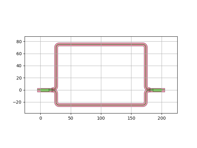
Instantiating and visualizing the MZI
mzi = ThermalMZI(name="thermalMZI")
mzi_lo = mzi.Layout()
mzi_lo.visualize()

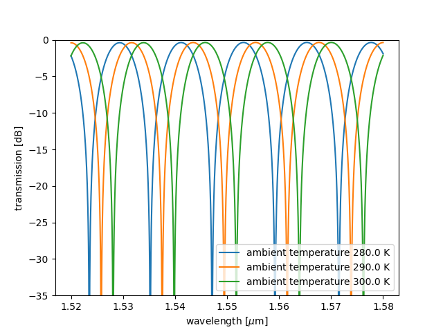
Running the Caphe simulation
We see that increasing temperature results in a redshift (longer wavelengths) of the transmission spectrum.
mzi_model = mzi.CircuitModel()
wavelength_range = np.linspace(1.52, 1.58, 1000)
temperature_range = np.linspace(280, 300, 3)

ax = plt.gca()
for T in temperature_range:
    s_matrix = mzi_model.get_smatrix(wavelength_range, temperature=T)
    ax.plot(wavelength_range, i3.signal_power_dB(s_matrix["out", "in"]), label=f"ambient temperature {T} K")

plt.legend()
plt.xlabel(r"wavelength [$\mu$m]")
plt.ylabel("transmission [dB]")
ax.set_ylim(-35, 0)
plt.show()
