3. PCell: Circuit Model

In the previous section, you have learned how to define the layout of an MMI. Now we will teach you how to add a circuit model to the MMI PCell. This circuit model will be used later to perform the simulation of a circuit containing several components.

The starting point is the MMI1x2 PCell explained in the previous section. This PCell contains layout information about the MMI, but so far we haven’t specified how the MMI should be simulated. This is done by adding

• a Netlist View, and

• a Circuit Model View

to the MMI. Let’s discover how to do this.

3.1. Netlist View

The goal of a Netlist is to define the interconnectivity between different cells (components). Interconnected PCells exchange information through optical or electrical signals, and are often connected with waveguides or electrical wires. Netlists contains all terms and connectivity information that is needed by Caphe, IPKISS’ circuit simulator, to create and simulate a circuit. The netlist can be specified manually or it can be extracted automatically from the Layout View. For more information about Netlists, check out our documentation: Netlist.

Our MMI doesn’t have any internal components nor connectivity and can just be described by the three terms (ports) that connect it to the outside world. When we defined the layout of our MMI, we exposed three ports (1 input and 2 outputs) using the _generate_ports method. Therefore, in this case, we can extract a netlist containing the terms of our MMI using i3.NetlistFromLayout.

pdks/si_fab/ipkiss/si_fab/components/mmi/pcell/cell.py

    class Netlist(i3.NetlistFromLayout):
        pass

3.2. Circuit Model View

Defining a circuit model for your components allows you to run circuit simulations and create a better understanding of the time and frequency behavior of your opto-electronic circuit. These circuit simulations rely on behavioral models for each of the devices in the circuit. A behavioral model allows to simulate the circuit sufficiently fast without losing too much accuracy. Instead of running a full physical simulation (such as Finite Difference Time Domain or Beam Propagation Method), the device is represented by a more approximate but faster model, such as a set of differential equations or a scattering matrix (S-matrix). For more information about circuit models, check out our documentation: Circuit models - Basics.

3.2.1. Defining the S-matrix

For a specific component, the S-matrix defines the amplitude and phase relationship between input and output signals in each term and for each mode. It is therefore an (m x n, m x n) square matrix as illustrated here.

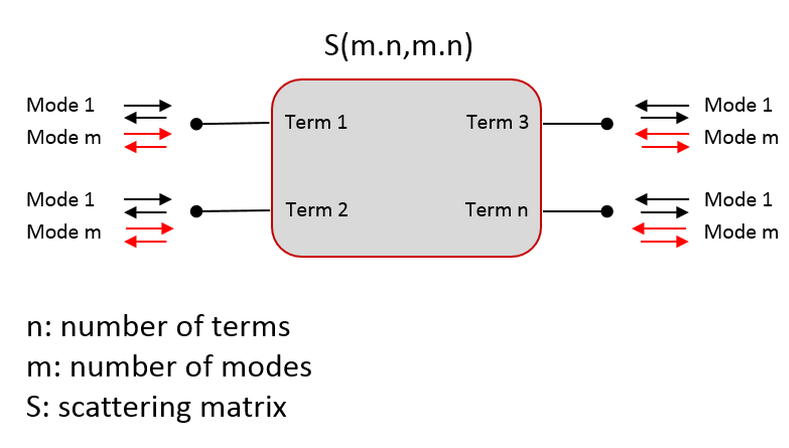
Our MMI has 3 terms and 1 mode per term. Therefore, we need 9 coefficients to define its S-matrix.

\[\begin{split}\left(\begin{array}{c} B_{in1}\\ B_{out1}\\ B_{out2} \end{array}\right)=\left(\begin{array}{cc} R_{in} & T_1 & T_2 \\ T_1 & R_{out1} & 0 \\ T_2 & 0 & R_{out2} \\ \end{array}\right)\left(\begin{array}{c} A_{in1}\\ A_{out1}\\ A_{out2} \end{array}\right)\end{split}\]

where:

• \(A_x\) denotes the incoming wave in each port;

• \(B_x\) denotes the outgoing wave from each port;

• \(T_1\) and \(T_2\) are the transmission coefficients from port in1 to ports out1 and out2, respectively;

• \(R_{in}\), \(R_{out1}\) and \(R_{out2}\) are the reflection coefficients at each port.

Our MMI is symmetrical, therefore \(T_1 = T_2 = T\) and \(R_{out1} = R_{out2} = R_{out}\). The S-matrix becomes:

\[\begin{split}\left(\begin{array}{c} B_{in1}\\ B_{out1}\\ B_{out2} \end{array}\right)=\left(\begin{array}{cc} R_{in} & T & T \\ T & R_{out} & 0 \\ T & 0 & R_{out} \\ \end{array}\right)\left(\begin{array}{c} A_{in1}\\ A_{out1}\\ A_{out2} \end{array}\right)\end{split}\]

3.2.2. Implementing the compact model

Using the S-matrix description we just defined, we can now implement a compact model for our MMI. This is usually done in a separate file from the one where you define a PCell. In case you want to build your own PDK or component library, we advise to store all the compact models of your components in one common file.

pdks/si_fab/ipkiss/si_fab/compactmodels/all.py

class MMI1x2Model(CompactModel):
    """Model for a 1x2 MMI.
    * center_wavelength: the center wavelength at which the device operates
    * reflection_in: polynomial coefficients relating reflection at the input port and wavelength
    * reflection_out: polynomial coefficients relating reflection at the output ports and wavelength
    * transmission: polynomial coefficients relating transmission and wavelength
    """

    parameters = [
        "center_wavelength",
        "reflection_in",
        "reflection_out",
        "transmission",
    ]

    terms = [
        OpticalTerm(name="in1"),
        OpticalTerm(name="out1"),
        OpticalTerm(name="out2"),
    ]

    def calculate_smatrix(parameters, env, S):
        reflection_in = np.polyval(parameters.reflection_in, env.wavelength - parameters.center_wavelength)
        reflection_out = np.polyval(parameters.reflection_out, env.wavelength - parameters.center_wavelength)
        transmission = np.polyval(parameters.transmission, env.wavelength - parameters.center_wavelength)
        S["in1", "out1"] = S["out1", "in1"] = transmission
        S["in1", "out2"] = S["out2", "in1"] = transmission
        S["in1", "in1"] = reflection_in
        S["out1", "out1"] = S["out2", "out2"] = reflection_out

Let’s analyze the code above:

1. Parameters. parameters lists the names of the variables that can change value and on which our S-matrix depends. In our case, we want to feed to the model the center wavelength at which we want to operate the device and polynomial coefficients that we use to calculate the transmission and the reflections. We will get back on this in a few moments.

2. Terms. In terms we declare the terminals of our model. In our case, we have one input and two outputs, for a total of three terms.

3. S-matrix calculation. In the calculate_smatrix function, we describe the frequency-domain response of our component by setting the elements of the S-matrix S. In our case, the reflection and transmission values are calculated by evaluating the polynomial coefficients provided as input in parameters at the desired wavelength values, centered at the center wavelength. The evaluation is performed using numpy.polyval().

   The idea behind feeding polynomial coefficients rather than absolute values of transmission and reflection obtained from a simulation is to make the model lighter. Instead of storing a large amount of data, containing reflection and transmission values at each desired wavelength, you can perform a fitting of this simulation data and store only a few coefficients that can be used to extract the transmission and the reflection at the desired wavelength.

4. Environment variables. In the method to calculate the S-matrix, env stands for the environment. It contains variables that are globally defined, such as the wavelength, frequency (c/wavelength), temperature. Currently this object only holds the wavelength and temperature variables, but this can be extended by the user defining the simulation.

A model of the time-domain response can also be added in the compact model of your component. However, we are not going to address this here. For more information about time-domain simulations, you can look at our documentation: Adding time domain behaviour.

3.2.3. Adding the circuit model to the PCell

The next step is to add a Circuit Model View to the MMI1x2 PCell.

pdks/si_fab/ipkiss/si_fab/components/mmi/pcell/cell.py

    class CircuitModel(i3.CircuitModelView):
        center_wavelength = i3.PositiveNumberProperty(doc="Center wavelength")
        transmission = i3.NumpyArrayProperty(doc="Polynomial coefficients, transmission as a function of wavelength")
        reflection_in = i3.NumpyArrayProperty(
            doc="Polynomial coefficients, reflection at input port as a function of wavelength"
        )
        reflection_out = i3.NumpyArrayProperty(
            doc="Polynomial coefficients, reflection at output ports as a function  of wavelength"
        )

        def _default_center_wavelength(self):
            raise NotImplementedError("Please specify center_wavelength")

        def _default_transmission(self):
            raise NotImplementedError("Please specify transmission")

        def _default_reflection_in(self):
            raise NotImplementedError("Please specify reflection_in")

        def _default_reflection_out(self):
            raise NotImplementedError("Please specify reflection_out")

        def _generate_model(self):
            return MMI1x2Model(
                center_wavelength=self.center_wavelength,
                transmission=self.transmission,
                reflection_in=self.reflection_in,
                reflection_out=self.reflection_out,

Let’s analyze this piece of code:

1. Properties. We defined a list of properties that we need for our model. These properties correspond to the list of parameters that we defined in the compact model. We assigned default values that are used in case the user doesn’t define these properties. Because we haven’t performed any optimization of our component, the default values are set to have no transmission and 100% reflection at each port.

2. Generate model. In the _generate_model method, we use the compact model we defined before, MMI1x2Model, to obtain the S-matrix of our component. When using this model, we pass the values of the center wavelength and of the coefficients of transmission and reflection from the properties of the CircuitModel class. As for the layout, this is done using self.<name_of_property>.

3.3. Instantiate the PCell

Now we can instantiate an MMI using MMI1x2 and perform a circuit simulation. First, we instantiate the MMI and its Layout View, as we did in the section about designing an MMI.

training/topical_training/device_optimization_mmi/explore_mmi_circuit_model.py

mmi = pdk.MMI1x2(
    trace_template=pdk.SiWireWaveguideTemplate(),
    width=5.0,
    length=15.0,
    taper_width=1.5,
    taper_length=4.0,
    waveguide_spacing=2.5,
)
mmi_lv = mmi.Layout()
mmi_lv.visualize(annotate=True)

Next, we choose the center wavelength and instantiate the Circuit Model View of the MMI. Because we haven’t performed any simulation, we assign dummy values to the transmission and reflection. Our list of coefficients contains only one value, which is the intercept of the polynomial. This means that the transmission and reflection are independent of the wavelength.

training/topical_training/device_optimization_mmi/explore_mmi_circuit_model.py

center_wavelength = 1.55
mmi_cm = mmi.CircuitModel(
    center_wavelength=center_wavelength,
    transmission=np.array([0.45**0.5]),
    reflection_in=np.array([0.01**0.5]),
    reflection_out=np.array([0.01**0.5]),
)

Finally, we define the wavelength range for our simulation, extract the S-matrix from the circuit model and plot the results. Here, we are plotting the transmission from port in1 to the out1 and out2 ports, and the reflection at the input port (in1).

training/topical_training/device_optimization_mmi/explore_mmi_circuit_model.py

wavelengths = np.linspace(1.5, 1.6, 51)
S = mmi_cm.get_smatrix(wavelengths=wavelengths)
S.visualize(
    term_pairs=[
        ("in1", "out1"),  # transmission 1
        ("in1", "out2"),  # transmission 2
        ("in1", "in1"),  # reflection
    ],
    scale="dB",
    yrange=(-30, 0),
)

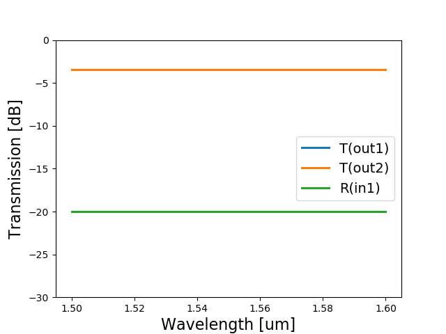
As expected, the response is the same at every wavelength. Because we provided values of transmission and reflection manually, this simulation doesn’t have physical meaning. The simulation results are not linked to the layout of our component.

In the next section, we are going to see how to optimize the MMI using CAMFR, a 2D mode solver included in IPKISS, and how to use the results of the CAMFR simulation in our circuit simulation. This will allow us to obtain a simulation linked to the physical parameters of the MMI.