MMI: Enriching PDK Components with Simulated Models
Note
This tutorial requires an installation of the Luceda Link for Ansys Lumerical. Please contact us for a trial license. For more detail on how to perform physical device simulation in Luceda IPKISS, please follow the Physical Device Simulation Flow tutorial, in particular the section on Interfacing with Lumerical MODE (EME).
This tutorial also requires the Luceda PDK for CORNERSTONE SiN, which is downloaded together with the Luceda Academy samples.
Introduction
The Luceda Photonics Design Platform is particularly well suited for creating coherent libraries of components that contain information about the following:
How to Layout the component through the LayoutView
How to Model the behaviour of the component in a circuit through the CircuitModelView
How to Simulate the behaviour of the component using IPKISS simulation recipes and third party solvers such as Ansys Lumerical
Because we don’t live in an ideal world, photonic design teams often find that the information which is shared by the foundry needs to be augmented by physical simulations. This is certainly the case for PDK components that contain only layout information, which is common for parametric cells.
In this tutorial, we will enrich an MMI from the Luceda PDK for CORNERSTONE SiN with both the following things:
A simulation recipe that uses Ansys Lumerical Lumerical MODE
A model for an optimized (and fixed) MMI
The enriched component will be added to a library called pteam_library_cornerstone_sin, which is a custom component library that targets the Luceda PDK for CORNERSTONE SiN. That component can in turn be used in circuit designs and be part of a Caphe circuit simulation.
Defining and using a simulation recipe for the MMI
Currently, the MMIs in the Cornerstone SiN PDK do not contain simulation recipes. Therefore, we will implement them ourselves in a custom library, called pteam_library_cornerstone_sin, which is based on the Cornerstone SiN technology and built on top of the Cornerstone SiN PDK. We create a component folder for the MMI and we organize all the information we need to store and document in the following sub-folders:
pteam_library_cornerstone_sin
    ├── compactmodels
    └── components
        └── mmi
            ├── data
            ├── pcell
            ├── regeneration
            ├── simulation
            └── __init__.py
data: It contains the simulated, or measured, S-matrix data that is used to model the designed component when running circuit simulations.pcell: This is the core of the component. It contains the PCell definition and, if needed, other utilities used to design the component.regeneration: It contains a regeneration script to regenerate simulation data of the optimized component. This is useful to ensure the S-matrix stored in thedatafolder is always up-to-date with the MMI layout.simulation: It contains the simulation recipe of the component.
In this tutorial, we define a simulation recipe that uses Lumerical MODE via our link with Ansys Lumerical.
This simulation recipe is added to the simulation subfolder, in a file called simulate_lumerical.py
We show the code for this simulation recipe below which is inspired by the code in the following tutorial (Ansys Lumerical MODE (EME)).
# Simulation recipe
def simulate_mmi_with_lumerical_eme(layout, wavelength_range, mesh_cells_y=200, project_folder="", data_tag=""):
    """Simulates a 2x1 MMI and returns it's transmission and reflections for the given layout, wavelength range and
    number of mesh cells.

    Parameters
    ----------
    layout: i3.LayoutView
        The layout of the given MMI
    wavelength_range: tuple
        The wavelength range in which it is simulated, in the format (minimum, maximum, number of wavelengths)
    mesh_cells_y: int, default=200, optional
        The number of transverse mesh cells along the y-dimension
    project_folder: str, default='', optional
        Folder to save the simulation data (S-matrix)
    data_tag: str, default=''
        String used to identify the saved simulation data of this component

    Returns
    -------
    transmission:
        The transmission of the MMI from any input port to the output port or vice versa
    reflection_in_same:
        The back reflection out of the same input port
    reflection_in_cross:
        The reflection out of a different input port
    reflection_out:
        The reflection at the output port
    """

    size_info = layout.size_info()

    sim_geom = i3.device_sim.SimulationGeometry(
        layout=layout,
        process_flow=i3.TECH.VFABRICATION.PROCESS_FLOW_SIN300_SIM,
        bounding_box=[
            None,  # x-span of the bounding box, here we use the default calculated by IPKISS
            [size_info.south - 3.0, size_info.north + 3.0],  # y-span of the bounding box
            None,  # z-span of the bbox, here we use the default calculated by IPKISS
        ],
    )

    simulation = i3.device_sim.LumericalEMESimulation(
        geometry=sim_geom,
        outputs=[
            i3.device_sim.SMatrixOutput(
                name="smatrix_" + data_tag,
                wavelength_range=wavelength_range,
            )
        ],
        setup_macros=[
            i3.device_sim.lumerical_macros.eme_transverse_mesh(mesh_cells_y=mesh_cells_y),
            i3.device_sim.lumerical_macros.eme_setup(
                group_spans=[layout.transition_length, layout.length, layout.transition_length],
                cells=[50, 1, 50],
            ),
            i3.device_sim.lumerical_macros.eme_profile_xy("out"),
        ],
        project_folder=project_folder,
        verbose=True,
        headless=False,
    )

    smatrix = simulation.get_result(name="smatrix_" + data_tag)

    transmission = np.abs(smatrix["out", "in1"])
    reflection_in_same = np.abs(smatrix["in1", "in1"])
    reflection_in_cross = np.abs(smatrix["in2", "in1"])
    reflection_out = np.abs(smatrix["out", "out"])

    return transmission, reflection_in_same, reflection_in_cross, reflection_out
This recipe is in the form of a function (simulate_mmi_with_lumerical_eme) that takes as an argument the layout of the component together with the range of wavelengths in which you wish to simulate it, followed by whichever optional arguments you wish to add.
This is the standard convention for defining a simulation recipe.
By using this convention, you will be able to simulate your devices using a consistent API throughout your project.
We take advantage of symmetry to store all the transmission and reflection data on our MMI in as few variables as possible. In particular, the propagation from either of the input ports to the output port is the same, as is propagation in the opposite direction. Information on all of them is thus stored in the same variable.
Now, using our simulation recipe to simulate the MMI is very straightforward. You only need to use the following code:
# Create and layout MMI from the Cornerstone library
mmi = pdk.STRIP_2x1_MMI()

mmi_layout = mmi.Layout(
    length=mmi_length,
    mmi_width=mmi_width,
    transition_length=taper_length,
    trace_spacing=waveguide_spacing,
)

# Simulate the MMI with Lumerical EME
wavelengths_start = center_wavelength - 0.05
wavelengths_end = center_wavelength + 0.05

# Note that the simulated results are artificial results as they're based on fictional technology
# and components. They only serve demonstration purposes.

transmission, reflection_in_same, reflection_in_cross, reflection_out = simulate_mmi_with_lumerical_eme(
    layout=mmi_layout,
    wavelength_range=(wavelengths_start, wavelengths_end, number_of_wavelengths),
    mesh_cells_y=mesh_size,
    project_folder=project_folder,
)
Test your knowledge
Check the file in training/topical_training/mmi_mode_simulation_eme/execute_mmi_simulation_recipe.py and try to answer the following question:
How does the mesh size affect simulation speed and accuracy?
Reduce the (transverse) mesh size to somewhere between 50-100 and check the impact on simulation speed.
Is the result the same as before?
Defining a circuit model for a (fixed) MMI
Now that we have implemented a simulation recipe, we will define a circuit model for an MMI that can use the results of this simulation.
The first step is to implement a compact model which describes the behaviour of the component (compactmodels/mmi.py).
The second step is to define a fixed PCell that uses the compact model (components/mmi/pcell/pcell.py).
The third step is to define a regeneration script that can run the simulation recipe on the fixed PCell and return the data required by the compact model of the fixed cell (components/mmi/regeneration/regenerate_strip_21_fixed.py).
A logical and well-structured organization of the library is important. We show the detailed file structure of this library below, with a few minor omissions.
pteam_library_si_fab
└── ipkiss
    └── pteam_library_si_fab
        ├── components
        │   ├── mmi
        │   │   ├── data
        │   │   ├── pcell
        │   │   │   ├── __init__.py
        │   │   │   ├── cell.py
        │   │   │   └── cell_utils.py
        │   │   ├── regeneration
        │   │   │   ├── __init__.py
        │   │   │   ├── regen_utils.py
        │   │   │   └── regenerate_strip_21_fixed.py
        │   │   ├── simulation
        │   │   │   ├── __init__.py
        │   │   │   └── simulate_lumerical.py
        │   │   └── __init__.py
        │   └── __init__.py
        │
        ├── compactmodels
        │   ├── mmi.py
        │   └── __init__.py
        │
        ├── __init__.py
        └── all.py
Step 1: Implementing a compact model
In our library, we store our model in a different folder from our components.
We call this folder compactmodels.
Let’s take a look at the compact model for the 2x1 MMI below:
from ipkiss3.pcell.model import CompactModel
from ipkiss3.pcell.photonics.term import OpticalTerm
import numpy as np


class MMI2x1Model(CompactModel):
    """Model for a 2x1 MMI.
    * center_wavelength: the center wavelength at which the device operates
    * transmission: polynomial coefficients relating transmission and wavelength
    * reflection_in_same: polynomial coefficients relating reflection at the input ports and wavelength
    * reflection_in_same: polynomial coefficients relating reflection between the input ports and wavelength
    * reflection_out: polynomial coefficients relating reflection at the output port and wavelength
    """

    parameters = [
        "center_wavelength",
        "transmission",
        "reflection_in_same",
        "reflection_in_cross",
        "reflection_out",
    ]

    terms = [
        OpticalTerm(name="in1"),
        OpticalTerm(name="in2"),
        OpticalTerm(name="out"),
    ]

    def calculate_smatrix(parameters, env, S):
        transmission = np.polyval(parameters.transmission, env.wavelength - parameters.center_wavelength)
        reflection_in_same = np.polyval(parameters.reflection_in_same, env.wavelength - parameters.center_wavelength)
        reflection_in_cross = np.polyval(parameters.reflection_in_cross, env.wavelength - parameters.center_wavelength)
        reflection_out = np.polyval(parameters.reflection_out, env.wavelength - parameters.center_wavelength)
        S["in1", "out"] = S["out", "in1"] = transmission
        S["in2", "out"] = S["out", "in2"] = transmission
        S["in1", "in1"] = S["in2", "in2"] = reflection_in_same
        S["in1", "in2"] = S["in2", "in1"] = reflection_in_cross
        S["out", "out"] = S["out", "out"] = reflection_out
Our compact model inherits from the class CompactModel in Luceda IPKISS.
All compact models in IPKISS do so.
We then list the parameters as a list of names inside the parameters variable.
In this case, the parameters are the polynomial coefficients for the transmission and the reflection at the different ports of the MMI.
Step 2: Define a fixed PCell
Now, we are ready to use the compact model in the circuit model view of the MMI PCell.
Since STRIP_2x1_MMI in the CORNERSTONE SiN PDK does not currently have a wavelength-dependent circuit model, we create a new PCell in our library to which we add a circuit model:
# PCell for a specific set of parameters


@i3.lock_properties()
class Strip2x1MMIFixed(pdk.STRIP_2x1_MMI):
    data_tag = i3.StringProperty(
        default="strip2x1_mmi",
        doc="String used to recognize the data in regeneration recipes",
    )

    def _default_data_tag(self):
        return "strip_2x1_mmi_fixed"

    class Layout(pdk.STRIP_2x1_MMI.Layout):
        def _default_length(self):
            return 129.0

        def _default_mmi_width(self):
            return 15.0

        def _default_transition_length(self):
            return 30.0

        def _default_trace_spacing(self):
            return 7.6

    class CircuitModel(i3.CircuitModelView):
        center_wavelength = i3.PositiveNumberProperty(doc="Center wavelength")
        transmission = i3.NumpyArrayProperty(doc="Polynomial coefficients, transmission as a function of wavelength")
        reflection_in_same = i3.NumpyArrayProperty(
            doc="Polynomial coefficients, reflection at input port as a function of wavelength",
        )
        reflection_in_cross = i3.NumpyArrayProperty(
            doc="Polynomial coefficients, reflection from one input port to the other as a function of wavelength",
        )
        reflection_out = i3.NumpyArrayProperty(
            doc="Polynomial coefficients, reflection at output ports as a function of wavelength",
        )

        @i3.cache()
        def _get_data(self):
            return get_data(self.data_tag)

        def _default_center_wavelength(self):
            c_wl, _, _, _, _ = self._get_data()
            return c_wl

        def _default_transmission(self):
            _, trans, _, _, _ = self._get_data()
            return trans

        def _default_reflection_in_same(self):
            _, _, refl_in_same, _, _ = self._get_data()
            return refl_in_same

        def _default_reflection_in_cross(self):
            _, _, _, refl_in_cross, _ = self._get_data()
            return refl_in_cross

        def _default_reflection_out(self):
            _, _, _, _, refl_out = self._get_data()
            return refl_out

        def _generate_model(self):
            return MMI2x1Model(
                center_wavelength=self.center_wavelength,
                transmission=self.transmission,
                reflection_in_same=self.reflection_in_same,
                reflection_in_cross=self.reflection_in_cross,
                reflection_out=self.reflection_out,
            )
The key observation here is that the cell Strip2x1MMIFixed inherits from the original PDK cell STRIP_2x1_MMI and adds a model based on data that is stored in pteam_library_cornerstone_sin/components/mmi/data/strip_2x1_mmi_fixed.z.
Now Strip2x1MMIFixed can be imported and used in a circuit simulation:
from cornerstone_sin import all as pdk # noqa: F401
from ipkiss3 import all as i3
from pteam_library_cornerstone_sin.all import Strip2x1MMIFixed
import numpy as np
import matplotlib.pyplot as plt
# Simulation wavelengths
sim_wavelengths = np.linspace(1.5, 1.6, 101)
# Simulate the MMI using the compact model, this time use PCell with hardcoded parameters
mmi = Strip2x1MMIFixed()
mmi_cm = mmi.CircuitModel()
# Simulate the MMI using the compact model
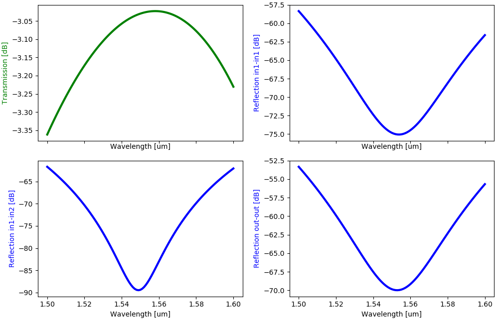
smatrix = mmi_cm.get_smatrix(wavelengths=sim_wavelengths)
wavelengths = smatrix.sweep_parameter_values
We obtain the following simulation results:
All we have left to do now is to define a script that regenerates the simulation data contained in pteam_library_cornerstone_sin/components/mmi/data/strip_2x1_mmi_fixed.z.
Step 3: The regeneration script
The goal of the regeneration script is to
simulate the fixed PCell
Strip2x1MMIFixed,perform a polynomial fit of the simulation data (transmission as a function of wavelength, reflection as a function of wavelength),
and store the polynomial coefficients in a file so that we can then re-use them when we build our circuit model.
Please note that this model will only be valid in the wavelength range that we have simulated. The regeneration script is created in the ‘regeneration’ folder inside the MMI folder in our component library:
        # Calculate polynomial coefficients
        pol_trans = np.polyfit(wavelengths_array - center_wavelength, transmission, 3)
        pol_refl_in_same = np.polyfit(wavelengths_array - center_wavelength, reflection_in_same, 3)
        pol_refl_in_cross = np.polyfit(wavelengths_array - center_wavelength, reflection_in_cross, 3)
        pol_refl_out = np.polyfit(wavelengths_array - center_wavelength, reflection_out, 3)

        # Store the polynomial coefficients
        params_path = os.path.join(base_directory, data_tag + ".json")
        results_np = {
            "center_wavelength": center_wavelength,
            "pol_trans": pol_trans,
            "pol_refl_in_same": pol_refl_in_same,
            "pol_refl_in_cross": pol_refl_in_cross,
            "pol_refl_out": pol_refl_out,
        }

        def serialize_ndarray(obj):
            return obj.tolist() if isinstance(obj, np.ndarray) else obj

        with open(params_path, "w") as f:
            json.dump(results_np, f, sort_keys=True, default=serialize_ndarray, indent=2)
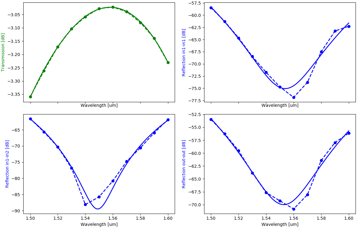
In the regeneration script, we also check how good our fitting is by plotting the fitted results alongside the simulation results:
    # Plotting
    if plot:
        params_path = os.path.join(base_directory, data_tag + ".json")

        with open(params_path) as f:
            results_np = json.load(f)

        wavelengths_fit = np.linspace(wavelengths[0], wavelengths[1], 1001)

        # Calculate fitted simulation results
        center_wavelength = results_np["center_wavelength"]
        transmission_fit = np.polyval(results_np["pol_trans"], wavelengths_fit - center_wavelength)
        reflection_in_same_fit = np.polyval(results_np["pol_refl_in_same"], wavelengths_fit - center_wavelength)
        reflection_in_cross_fit = np.polyval(results_np["pol_refl_in_cross"], wavelengths_fit - center_wavelength)
        reflection_out_fit = np.polyval(results_np["pol_refl_out"], wavelengths_fit - center_wavelength)

        # Plot simulation results
        def dB(x):
            return 20 * np.log10(np.abs(x))

        fig, axs = plt.subplots(nrows=2, ncols=2, sharex="col", constrained_layout=True)
        axs = axs.flatten()

        axs[0].plot(wavelengths_fit, dB(transmission_fit), label="transmission, fit", linewidth=2, color="g")
        axs[0].set_xlabel("Wavelength [um]")
        axs[0].set_ylabel("Transmission [dB]", color="g")

        axs[1].plot(
            wavelengths_fit, dB(reflection_in_same_fit), label="backreflection in1->in1, fit", linewidth=2, color="b"
        )
        axs[1].set_xlabel("Wavelength [um]")
        axs[1].set_ylabel("Reflection in1-in1 [dB]", color="b")

        axs[2].plot(
            wavelengths_fit, dB(reflection_in_cross_fit), label="backreflection in1->in2, fit", linewidth=2, color="b"
        )
        axs[2].set_xlabel("Wavelength [um]")
        axs[2].set_ylabel("Reflection in1-in2 [dB]", color="b")

        axs[3].plot(
            wavelengths_fit, dB(reflection_out_fit), label="backreflection out->out, fit", linewidth=2, color="b"
        )
        axs[3].set_xlabel("Wavelength [um]")
        axs[3].set_ylabel("Reflection out-out [dB]", color="b")

        if resimulate:
            axs[0].plot(
                wavelengths_array,
                dB(transmission),
                label="transmission, simulated",
                linewidth=2,
                color="g",
                marker="o",
                linestyle="--",
            )

            axs[1].plot(
                wavelengths_array,
                dB(reflection_in_same),
                label="backreflection in1->in1, simulated",
                linewidth=2,
                color="b",
                marker="o",
                linestyle="--",
            )

            axs[2].plot(
                wavelengths_array,
                dB(reflection_in_cross),
                label="backreflection in1->in2, simulated",
                linewidth=2,
                color="b",
                marker="o",
                linestyle="--",
            )

            axs[3].plot(
                wavelengths_array,
                dB(reflection_out),
                label="backreflection out->out, simulated",
                linewidth=2,
                color="b",
                marker="o",
                linestyle="--",
            )

        plt.show()
Try it out
Rerun pteam_library_cornerstone_sin/components/mmi/regeneration/regenerate_strip_21_fixed.py and wait until the simulation finishes.