AWG generation: Assembly
In the previous step we derived the implementation parameters from functional specifications. Now, we will assemble the AWG. This consists of three steps:
Implement the star couplers
Implement the waveguide array
Assemble the AWG and inspect
Defining the star couplers
First, we define the star couplers, starting from the output star coupler. This is broken down into four steps:
Add dummy apertures
Generate the aperture mounting, positioning the apertures in a Rowland or confocal configuration
Generate a contour drawing for the free propagation region
Compose the star coupler and inspect
The reason why these four steps have been defined is to give the designer a large degree of control over the details of the implementation.
Several utility functions are defined in the Luceda AWG Designer to support the user. The following code excerpt shows the implementation of the output star coupler. The input star coupler follows the same flow.
    # Output star coupler
    print("Defining output star coupler...\n")
    # Add dummies
    n_dummies = 2
    out_array, out_array_angles = awg.get_apertures_angles_with_dummies(
        apertures=[aperture] * n_arms,
        angles=angles_arms_out,
        n_dummies=n_dummies,
    )
    out_ports, out_ports_angles = awg.get_apertures_angles_with_dummies(
        apertures=[aperture] * len(angles_out),
        angles=angles_out,
        n_dummies=n_dummies,
    )

    # Generate aperture mounting
    out_array_aperture, out_ports_aperture, out_array_xforms, out_ports_xforms = awg.get_star_coupler_apertures(
        apertures_arms=out_array,
        apertures_ports=out_ports,
        angles_arms=out_array_angles,
        angles_ports=out_ports_angles,
        radius=grating_radius_output,
        mounting="rowland",
        input=False,
    )

    # Generate free propagation contour
    contour = awg.get_star_coupler_extended_contour(
        apertures_in=out_array,
        apertures_out=out_ports,
        trans_in=out_array_xforms,
        trans_out=out_ports_xforms,
        radius_in=grating_radius_output,
        radius_out=grating_radius_output * 0.5,
        extension_angles=(10, 10),
        aperture_extension=(0.0, 0.1),
        layers_in=[i3.TECH.PPLAYER.SI],
        layers_out=[i3.TECH.PPLAYER.SI, i3.TECH.PPLAYER.SHALLOW],
    )

    # Compose star coupler
    sc_out = awg.StarCoupler(
        aperture_in=out_array_aperture,
        aperture_out=out_ports_aperture,
    )
    sc_out.Layout(contour=contour)
    sc_out.CircuitModel(simulation_wavelengths=[1.3])
Note
We have set simulation_wavelengths=[1.3] on the apertures.
This limits the simulation of the apertures to a single wavelength, which is good enough for a first simulation.
If you want to simulate the apertures for each wavelength, then set simulation_wavelengths=None but keep in mind that the simulation can take a long time.
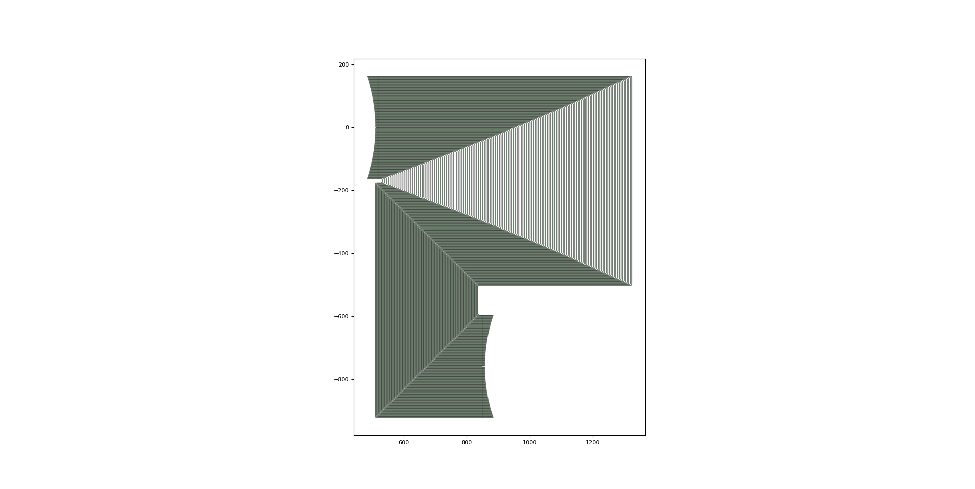
The virtual fabrication of the resulting output star coupler is:
Adding dummies
First, we create a list of apertures and their rotation angles, including a number of dummies. These dummies are important to make sure that the outer apertures see the same neighbours as the inner apertures. This affects both their fabrication (lithography, etching, planarization) and their optical behavior.
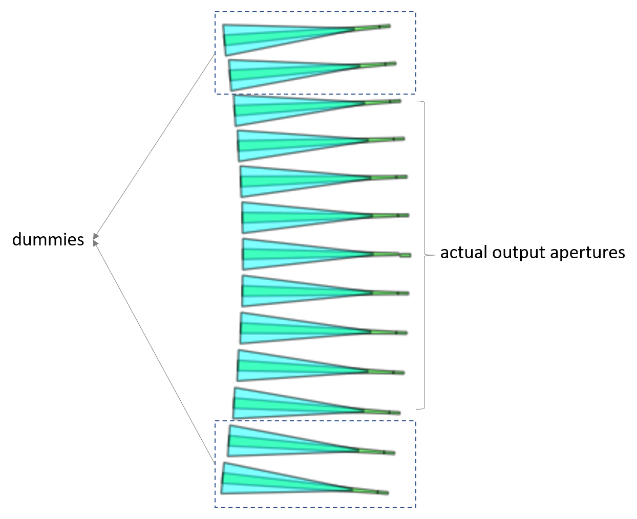
To that end, we call the AWG Designer’s function get_apertures_angles_with_dummies(apertures, angles, n_dummies), once for the input side and once for the output side.
This function returns the final list of apertures and a list of their angles.
Note that for simplicity we use a single aperture for the ports here.
In a real design you might want to optimize each aperture for the target wavelength it will capture.
    # Add dummies
    n_dummies = 2
    out_array, out_array_angles = awg.get_apertures_angles_with_dummies(
        apertures=[aperture] * n_arms,
        angles=angles_arms_out,
        n_dummies=n_dummies,
    )
    out_ports, out_ports_angles = awg.get_apertures_angles_with_dummies(
        apertures=[aperture] * len(angles_out),
        angles=angles_out,
        n_dummies=n_dummies,
    )
Generating the aperture mounting
Next, the apertures will be mounted in the desired configuration to form a star coupler. Out-of-the-box provided mountings are rowland or confocal.
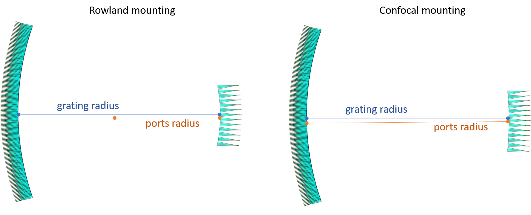
The AWG Designer provides the function get_star_coupler_apertures(apertures_arms, apertures_ports, angles_arms, angles_ports, radious, mounting, input) for this purpose.
This function returns two MultiAperture objects, one for the input side and one for the output side.
Multi-apertures are an internal functionality used to join a list of apertures into one object, facilitating simulation.
The function also returns their transformations (the input side will be mirrored compared to the array side).
    # Generate aperture mounting
    out_array_aperture, out_ports_aperture, out_array_xforms, out_ports_xforms = awg.get_star_coupler_apertures(
        apertures_arms=out_array,
        apertures_ports=out_ports,
        angles_arms=out_array_angles,
        angles_ports=out_ports_angles,
        radius=grating_radius_output,
        mounting="rowland",
        input=False,
    )
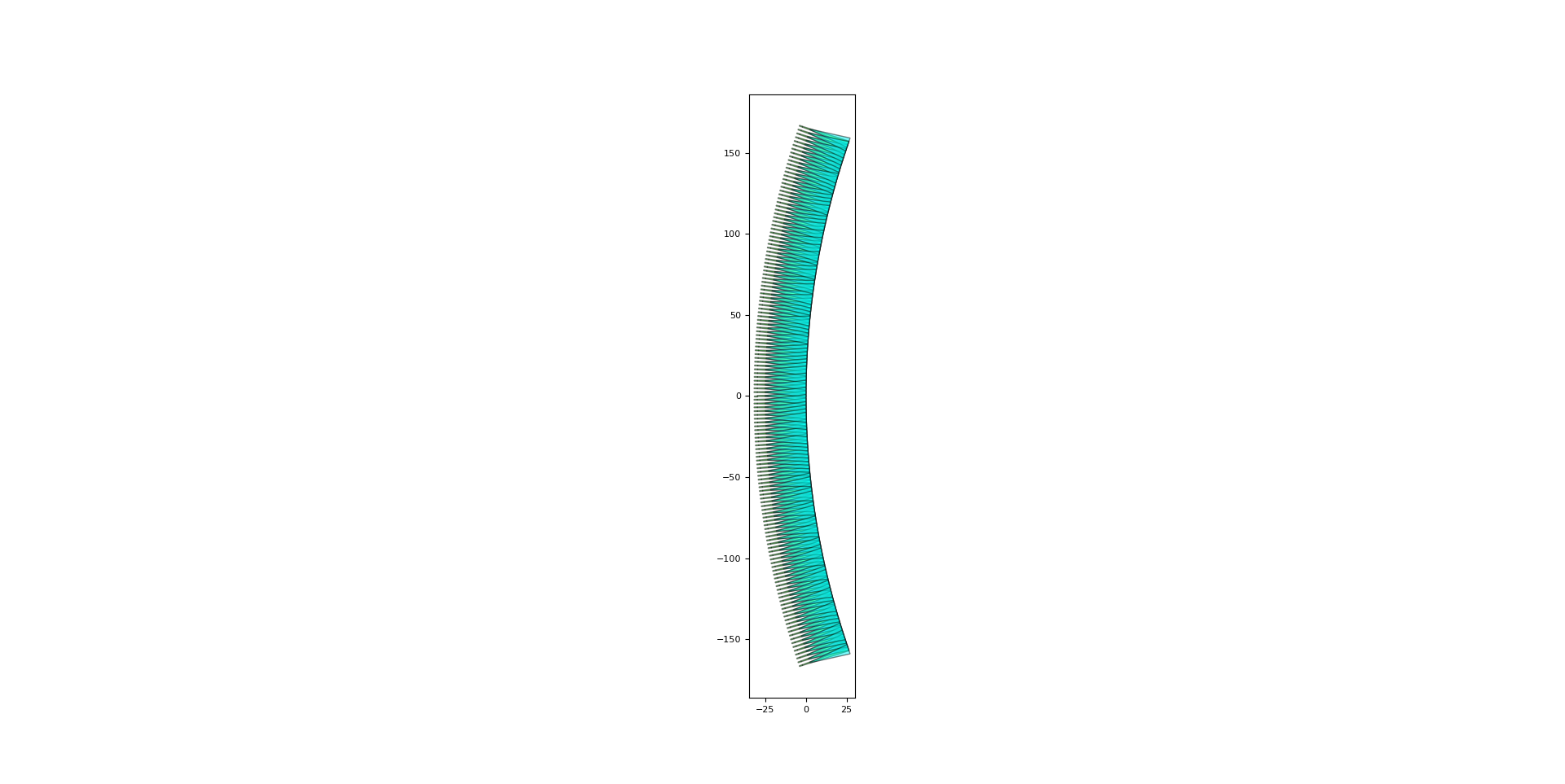
The resulting mounted multi-apertures are:
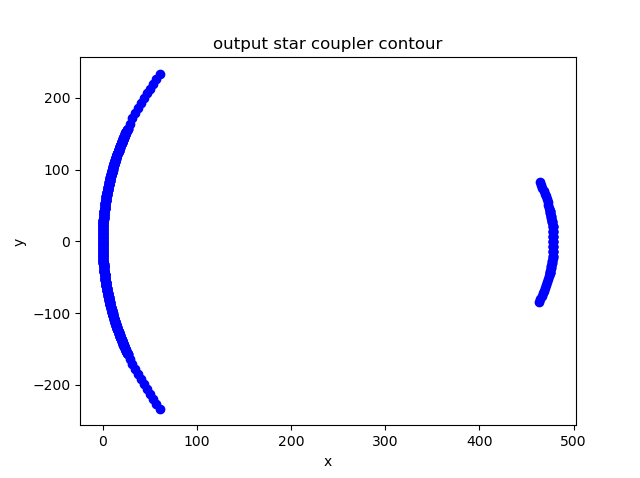
Generating the contour
Next, we need to draw the free propagation region to ensure this is a continuous piece of a slab waveguide.
In the case of SiFab technology, a drawing on the SI layer is needed (otherwise, all silicon would be etched away).
In addition, we need to ensure that this free propagation region contour perfectly matches the apertures.
To this end, we use the function get_star_coupler_extended_contour():
    # Generate free propagation contour
    contour = awg.get_star_coupler_extended_contour(
        apertures_in=out_array,
        apertures_out=out_ports,
        trans_in=out_array_xforms,
        trans_out=out_ports_xforms,
        radius_in=grating_radius_output,
        radius_out=grating_radius_output * 0.5,
        extension_angles=(10, 10),
        aperture_extension=(0.0, 0.1),
        layers_in=[i3.TECH.PPLAYER.SI],
        layers_out=[i3.TECH.PPLAYER.SI, i3.TECH.PPLAYER.SHALLOW],
    )
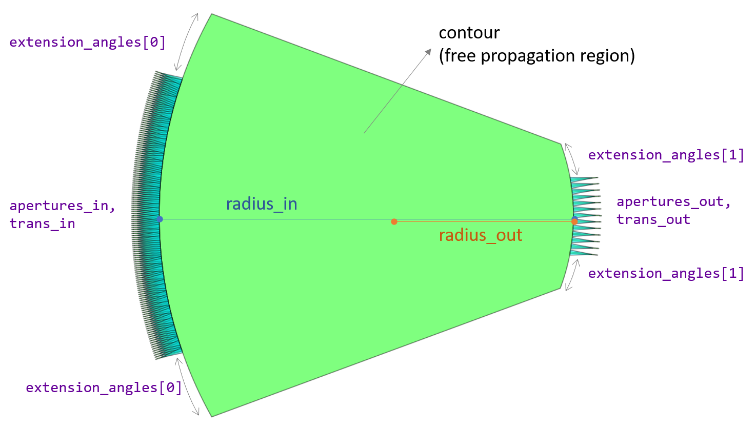
This function takes as inputs the mounted apertures generated in the previous step, and draws a contour which extends from them along a circle. Particularly during the first design iterations on a technology, drawing the contour a bit wider than the apertures can be important to avoid loss or reflections in case the light diffracts a bit wider than anticipated.
The
apertures_in,apertures_out,trans_in,trans_outarguments are the outputs of the previous step.The
radius_inis the radius of the circle of the extended drawing. For the output star coupler, this is the radius of the waveguide array aperture mounting.The radius of the outer side
radius_outcan be drawn differently. In this example we choose to follow the Rowland mounting where half the waveguide array radius is used.The argument
extension_anglesspecifies how far along the aperture circles we want the contour to extend. In this example, we choose 10 degrees for both the input and output side of the star coupler.The argument
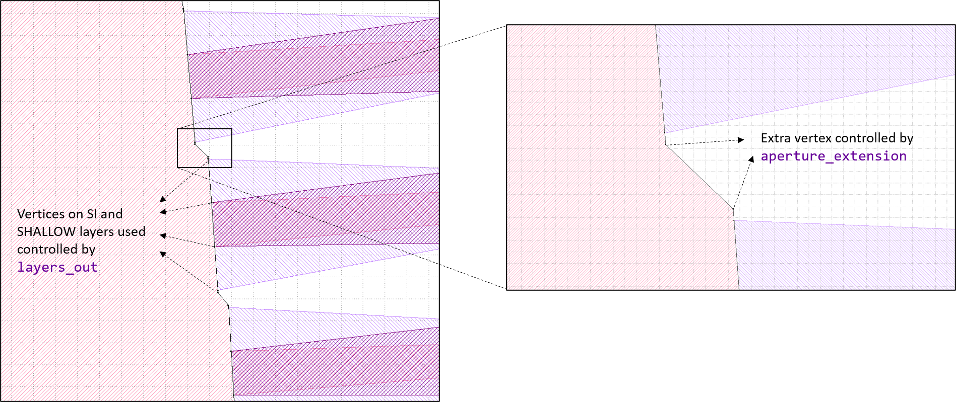
aperture_extensionallows us to specify the drawing of additional vertices in between the two apertures. On the waveguide array side, we want the apertures to be very close together so we don’t need an additional vertex drawn. On the ports side (output side of the output star coupler), we want an additional vertex drawn in order to make sure that the aperture’s opening into the FPR is not distorted by drawing the contour.
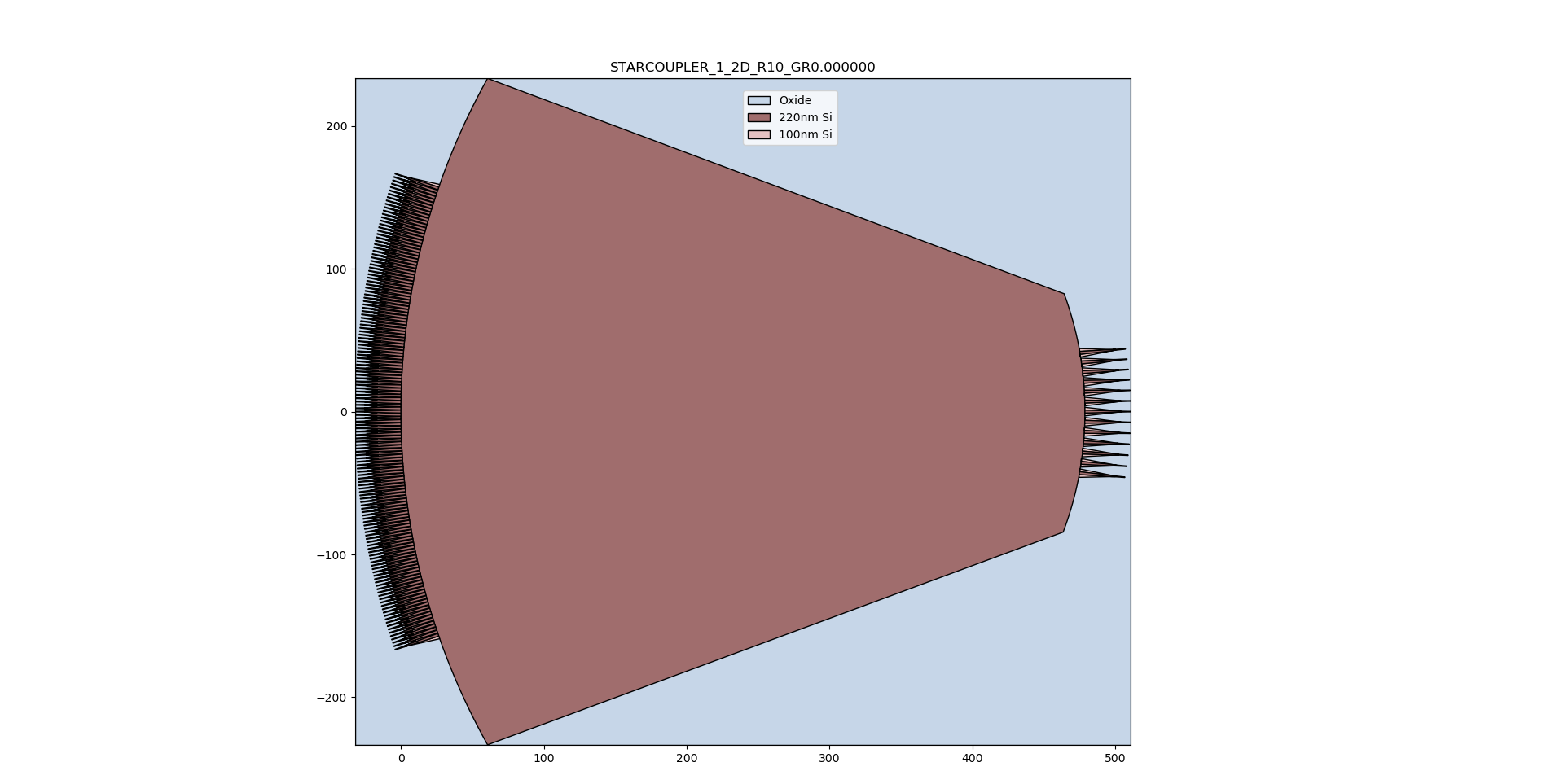
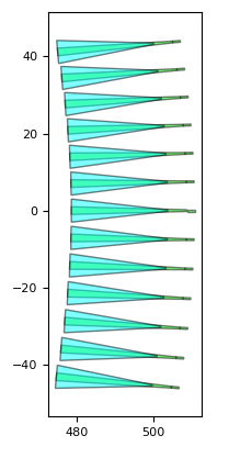
The resulting contour shape is:
Compose the star coupler
Finally, we are ready to put the pieces together in a StarCoupler object:
    # Compose star coupler
    sc_out = awg.StarCoupler(
        aperture_in=out_array_aperture,
        aperture_out=out_ports_aperture,
    )
    sc_out.Layout(contour=contour)
    sc_out.CircuitModel(simulation_wavelengths=[1.3])
Here, for the example’s sake, we set the parameter simulation_wavelengths of the star coupler’s circuit model to a single wavelength.
This will reduce the number of simulations needed to build up the model at the expense of less accurate results.
After the initial design iterations, it can be set to None in order to simulate the AWG completely.
Routing the waveguide array
Now that the star couplers are generated, we can create the waveguide array. For this purpose, we need to find a way to route the waveguides with the given star couplers and delay length. However, there are several constraints and trade-offs to consider:
We want to keep a certain minimum waveguide spacing in order to avoid coupling between the waveguides.
We want the AWG to be as compact as possible to reduce the ‘chip real estate’ used and to reduce the impact of fabrication variations (e.g. layer thickness).
In a silicon photonics foundry technology, we’d like to avoid implementing the delay length with curvilinear waveguides. Therefore, we prefer Manhattan-style routing to implement the delay length in the straight parts as much as possible.
The delay length of 6.75 um, which resulted form the synthesis, is relatively short compared to the minimum waveguide spacing.
Therefore, and because of the above considerations, we choose an S-shaped AWG.
This is provided out-of-the-box in the Luceda AWG Designer (SWaveguideArray):
    # Create the waveguide array
    print("Creating waveguide array...\n")
    delays = [delay_length * i for i in range(n_arms)]
    wg_array = awg.SWaveguideArray(
        start_ports=sc_in_layout.east_ports.y_sorted(),
        delay_lengths=delays,
    )
    wg_array.Layout(
        offset_output_ports_south=80.0,
        route_properties={
            "rounding_algorithm": i3.SplineRoundingAlgorithm(adiabatic_angles=(15.0, 15.0)),
        },
    )
The offset_output_ports_south argument will be clarified in the next step.
To minimize the bending losses, we use adiabatic bends.
We do this setting the argument route_properties to use i3.SplineRoundingAlgorithm as its rounding algorithm.
The result is the following waveguide array:
Note
In a different technology or for a different application, the constraints and trade-offs might be different. It is not difficult to implement your own custom waveguide array if it is not offered out-of-the-box by the Luceda AWG Designer yet. Alternatively, you can ask Luceda to help with the implementation by contacting us at support@lucedaphotonics.com.
AWG assembly
The final step of the implementation is probably the most straightforward:
we make an ArrayedWaveguideGrating object out of the input star coupler, output star coupler and waveguide array.
# Create AWG
print("Creating AWG...\n")
cwdm_awg = awg.ArrayedWaveguideGrating(
star_coupler_in=sc_in,
star_coupler_out=sc_out,
waveguide_array=wg_array,
)
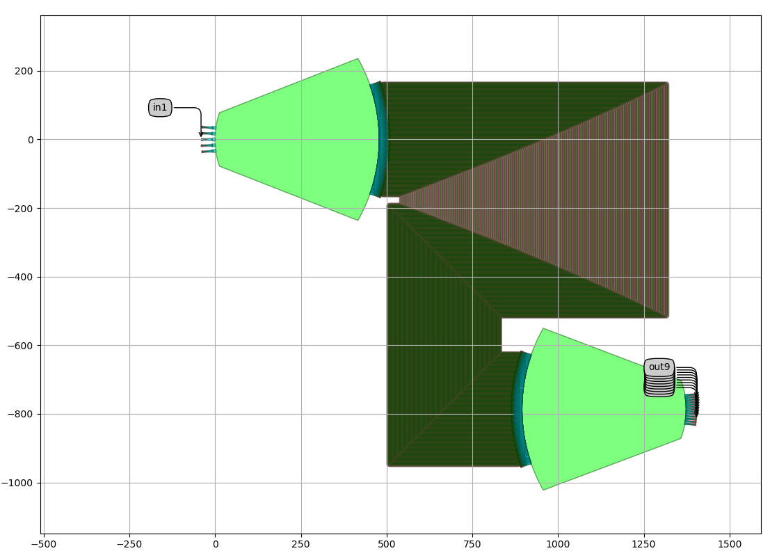
cwdm_awg_layout = cwdm_awg.Layout()
if plot:
cwdm_awg_layout.visualize(annotate=True)
if save_dir:
gds_path = os.path.abspath(os.path.join(save_dir, "awg_{}.gds".format(tag)))
cwdm_awg_layout.write_gdsii(gds_path)
print("{} written.".format(gds_path))
return cwdm_awg