AWG simulation and analysis
Simulation
At this point we have a complete AWG with a layout, a logical netlist and a simulation model.
We can now simply ask Caphe (Luceda IPKISS’ built-in circuit simulator) to calculate its S-parameters
and save the results.
This is done by the simulate_awg function that we have defined in rect_awg/simulate.py.
This function takes the AWG PCell and a set of wavelengths as input and returns the simulated S-matrix.
from ipkiss3 import all as i3
import os


def simulate_awg(awg, wavelengths, save_dir=None, tag=""):
    """Custom function to simulate an AWG. If you make an AWG, you should write one of your own.
    Parameters are the awg cell you want to simulate and things that control your simulation as well as
    parameters that control where you save your data.

    Parameters
    ----------
    awg : i3.Pcell
          AWG PCell
    wavelengths: ndarray
                 Simulation wavelengths
    save_dir: str, default: None, optional
              If specified, a GDSII file is saved in this directory
    tag: str, optional
         String used to give a name to saved files

    Returns
    -------
    awg_s:
           S-matrix of the simulated AWG

    """
    cwdm_awg_cm = awg.get_default_view(i3.CircuitModelView)
    print("Simulating AWG...\n")
    awg_s = cwdm_awg_cm.get_smatrix(wavelengths)
    if save_dir:
        smatrix_path = os.path.join(save_dir, "smatrix_{}.s{}p".format(tag, awg_s.data.shape[0]))
        awg_s.to_touchstone(smatrix_path)
        print("{} written".format(smatrix_path))
    return awg_s
Analysis
Next, the function analyze_awg, defined in rect_awg/analyze.py, will take the S-matrix and check it against the figure of merit.
In this analysis function we define the AWG specifications and check the behaviour of the AWG according to those specs, using helper functions provided in the Luceda AWG Designer.
Let’s have a look a the function signature.
def analyze_awg(awg_s, peak_threshold=-10.0, plot=True, save_dir=None, tag=""):
    """Custom AWG analysis function. If you make an AWG, you should write an analysis function of your own.
    The goal of the analyze_awg function is to answer the question: how does the AWG perform
    according to my specs? In an analysis function you define the specs and check the behaviour
    of the AWG according to those specs using helper functions provided in the Luceda AWG Designer.
    The parameters are the things you want to vary as well as options to control whether you
    plot and where you save your data.

    Parameters
    ----------
    awg_s: SMatrix1DSweep
        S-matrix of the AWG
    peak_threshold: float, default: -10.0, optional
        The power threshold for peak detection (in dB)
    plot: bool, default: True, optional
        If true, the spectrum is plotted
    save_dir: str, default: None, optional
        If specified, a GDSII file is saved in this directory
    tag: str, optional
        String used to give a name to saved files

    Returns
    ------
    report: dict
        Dictionary containing analysis specs
    """
Specifications
The first step of the analysis function is to define the specifications. Here we hard code the specifications of the required transmission channels. If necessary, parametric specifications may be inserted in the signature of the analysis function.
    # Specs
    channel_freq = np.array([229000.0, 229800.0, 230600.0, 231400.0, 232200.0, 233000.0, 233800.0, 234600.0, 235400.0])
    channel_wav = awg.frequency_to_wavelength(channel_freq)
    channel_width = 10e-4
    output_ports = ["out{}".format(p + 1) for p in range(len(channel_wav))]
Initialize the spectrum analyzer
The measurements are done using i3.SpectrumAnalyzer.
We initialize the spectrum analyzer with
the S-matrix data of the AWG,
the input port (or port:mode) to consider,
the output ports (or port:mode) which we want to analyze,
whether we want to analyze in dB scale (True) or linear (False),
and the threshold we set for deciding about peaks: -10 (dB) by default. We made this a parameter to
analyze_awg(see AWG finalization).
    # Initialize spectrum analyzer
    analyzer = i3.SpectrumAnalyzer(
        smatrix=awg_s,
        input_port_mode="in1:0",
        output_port_modes=output_ports,
        dB=True,
        peak_threshold=peak_threshold,
    )
    analyzer = analyzer.trim(
        (
            min(channel_wav) - channel_width,
            max(channel_wav) + channel_width,
        )
    )
Measure key parameters
Now we use the spectrum analyzer to measure different properties of the AWG we want to validate against specifications:
The peak wavelengths
The channel widths
The (minimum) insertion loss within the channel
The nearest-neighbour crosstalk
The crosstalk from further neighbours (excluding nearest-neighbour contributions)
The 3dB passbands of the channels
    # Measurements
    peaks = analyzer.peaks()
    peak_wavelengths = [peak["wavelength"][0] for peak in peaks.values()]
    peak_error = np.abs(channel_wav - peak_wavelengths)

    bands = analyzer.width_passbands(channel_width)
    insertion_loss = list(analyzer.min_insertion_losses(bands=bands).values())
    cross_talk_near = list(analyzer.near_crosstalk(bands=bands).values())
    cross_talk_far = list(analyzer.far_crosstalk(bands=bands).values())
    passbands_3dB = list(analyzer.cutoff_passbands(cutoff=-3.0).values())
Plotting and report generation
Next, we write a report containing the analyzed specifications. For later reference, this is stored in a file.
    # Create report
    report = dict()
    band_values = list(bands.values())
    for cnt, port in enumerate(output_ports):
        channel_report = {
            "peak_expected": channel_wav[cnt],
            "peak_simulated": peak_wavelengths[cnt],
            "peak_error": peak_error[cnt],
            "band": band_values[cnt][0],
            "insertion_loss": insertion_loss[cnt][0],
            "cross_talk": cross_talk_far[cnt] - insertion_loss[cnt][0],
            "cross_talk_nn": cross_talk_near[cnt] - insertion_loss[cnt][0],
            "passbands_3dB": passbands_3dB[cnt],
        }
        report[port] = channel_report

    if save_dir:

        def serialize_ndarray(obj):
            return obj.tolist() if isinstance(obj, np.ndarray) else obj

        report_path = os.path.join(save_dir, "report_{}.json".format(tag))
        with open(report_path, "w") as f:
            json.dump(report, f, sort_keys=True, default=serialize_ndarray, indent=0)
        print("{} written".format(report_path))
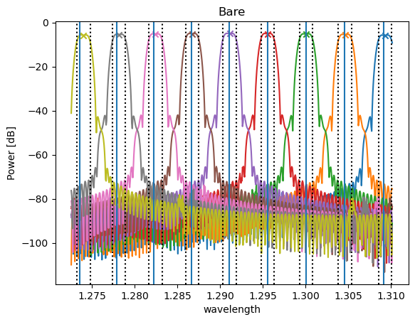
Finally, we plot the transmission spectrum and write a report.
    # Plot spectrum and specified channels
    fig = analyzer.visualize(title=tag.capitalize(), show=False)
    for spec_wavelength in channel_wav:
        plt.axvline(x=spec_wavelength)

    for passband in passbands_3dB:
        plt.axvline(x=passband[0][0], color="k", linestyle=":")
        plt.axvline(x=passband[0][1], color="k", linestyle=":")

    png_path = os.path.join(save_dir, "spectrum_{}.png".format(tag))
    fig.savefig(os.path.join(save_dir, png_path), bbox_inches="tight")
    print("{} written".format(png_path))

    if plot:
        # Plot transmission spectrum
        plt.show()
    plt.close(fig)
Report JSON file: report_finalized.json