Connectors
Connecting components is an important part of every integrated photonics design. In IPKISS, the easiest way to achieve this is by defining connectors inside the placement and routing specifications of your circuit. They provide information on what is connected in your circuit and how. More specifically, every connector creates a cell that automatically defines a waveguide connection between specified start and end ports.
In this section, we will first discuss the two main types of connectors to create optical waveguides: i3.ConnectBend and i3.ConnectManhattan.
After that, we will discuss how to chain multiple connectors and route bundles of connections.
Finally, the addendum of this section provides examples on fully customizing a connection bundle.
ConnectBend
The i3.ConnectBend connector creates the simplest possible bend between two optical ports, based on the given rounding parameters, port positions, and angles.
These rounding parameters are defined by the minimal bend_radius and rounding_algorithm of the bend.
For example, by using i3.ConnectBend in the code below, a U-bend connection is created between two grating couplers.
import si_fab.all as pdk
import ipkiss3.all as i3

# Define and instantiate grating couplers
gc = pdk.FC_TE_1550()
specs = [
    i3.Inst(["gc1", "gc2"], gc),
    i3.Place("gc1:out", (0, 150)),
    i3.Place("gc2:out", (0, 0)),
    i3.ConnectBend(
        "gc1:out",
        "gc2:out",
        bend_radius=10,
    ),
]

# Visualize circuit1
circuit1 = i3.Circuit(specs=specs)
circuit1_lo = circuit1.Layout()
circuit1_lo.visualize()
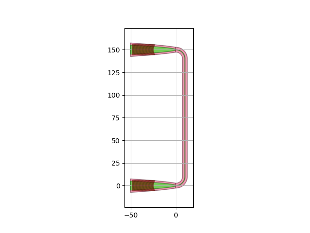
This bend follows the most simple route based on the given input parameters passed to the connector.
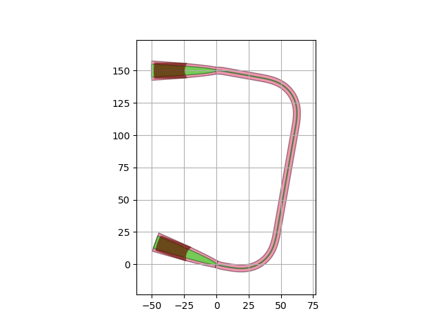
In the example below, you can see how the route changes when one of the grating couplers is rotated by 20°, the bend_radius parameter is set to 25 µm and the rounding algorithm is set to i3.EulerRoundingAlgorithm.
# Place and route grating couplers circuit2
specs = [
    i3.Inst(["gc1", "gc2"], gc),
    i3.Place("gc1:out", (0, 150)),
    i3.Place("gc2:out", (0, 0), angle=-20),
    i3.ConnectBend(
        "gc1:out",
        "gc2:out",
        bend_radius=25,
        rounding_algorithm=i3.EulerRoundingAlgorithm(),
    ),
]

# Visualize circuit2
circuit2 = i3.Circuit(specs=specs)
circuit2_lo = circuit2.Layout()
circuit2_lo.visualize()
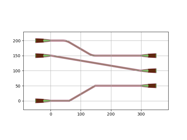
You can further refine the routing of your connection by using the parameters start_straight and end_straight inside this connector.
They define the length of the straight sections at the start and end of the connection.
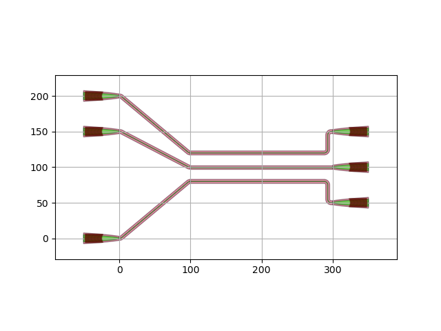
The code below shows how to use these parameters to create three connections between grating couplers.
import si_fab.all as pdk
import ipkiss3.all as i3

# Define and instantiate grating couplers
gc = pdk.FC_TE_1550()

# Placement of grating couplers
placement = [
    i3.Inst([f"gc_in{count}" for count in range(1, 4)], gc),
    i3.Inst([f"gc_out{count}" for count in range(1, 4)], gc),
    i3.Place("gc_in1:out", (0, 200)),
    i3.Place("gc_in2:out", (0, 150)),
    i3.Place("gc_in3:out", (0, 0)),
    i3.Place("gc_out1:out", (300, 150), angle=180),
    i3.Place("gc_out2:out", (300, 100), angle=180),
    i3.Place("gc_out3:out", (300, 50), angle=180),
]

# Routing specs of circuit1
route1 = [
    i3.ConnectBend(
        "gc_in1:out",
        "gc_out1:out",
        start_straight=40.0,
        end_straight=150,
        bend_radius=45.0,
    ),
    i3.ConnectBend(
        "gc_in2:out",
        "gc_out2:out",
    ),
    i3.ConnectBend(
        "gc_in3:out",
        "gc_out3:out",
        start_straight=60.0,
        end_straight=150,
    ),
]

# Create and visualize circuit1
specs = placement + route1
circuit1 = i3.Circuit(specs=specs)
circuit1_lo = circuit1.Layout()
circuit1_lo.visualize()
ConnectManhattan
Another type of connector is i3.ConnectManhattan.
This connector generates connections with 90° angles, navigating through horizontal and vertical lines.
If more control in the routing is desired, control points can be added as a list to the control_points parameter.
These control points can be specified using i3.V and i3.H, which route the connector through the specified x- and y-coordinates, respectively.
The same three connections between grating couplers can now be created using i3.ConnectManhattan connectors.
luceda_academy/training/topical_training/connectors_trace_templates_wg/1_connectors/1_2_connections_west_to_east.py# Routing specs of circuit2 route2 = [ i3.ConnectManhattan( "gc_in1:out", "gc_out1:out", ), i3.ConnectManhattan( "gc_in2:out", "gc_out2:out", control_points=[i3.V(100)], ), i3.ConnectManhattan( "gc_in3:out", "gc_out3:out", control_points=[i3.V(i3.START + 40), i3.H(25), i3.V(i3.END - 100)], ), ] # Create and visualize circuit2 specs = placement + route2 circuit2 = i3.Circuit(specs=specs) circuit2_lo = circuit2.Layout() circuit2_lo.visualize()
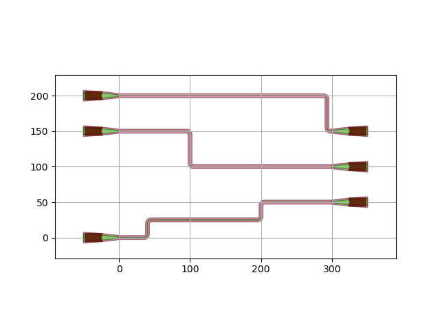
In the code above, some of the control points are defined in a relative way by using anchors.
An anchor is a point in space, which is tied to a location on a specific instance or a coordinate of a specific instance.
It can be tied to the edges, ports or corners of any instance.
The anchors used here are the start port (i3.START) and the end port (i3.END) of the connector.
A more detailed tutorial about using control points and anchors for placement and routing in your circuit can be found in Placement and routing specifications.
If you want to define your own anchors: have a look at i3.Anchor.
Chaining connectors
In some situations, more complex connections are needed that require multiple connectors to be combined together.
We can realize this by creating a chain of connectors.
In the example below, the connections between the grating couplers are created by combining a i3.ConnectBend with a i3.ConnectManhattan connector.
First, we define intermediate ports, which will be the points where the connectors will combine.
Don’t forget to name these intermediate ports.
Next, we define every connector individually inside the specs list of the circuit.
luceda_academy/training/topical_training/connectors_trace_templates_wg/1_connectors/1_2_connections_west_to_east.py# Define intermediate ports intermediate_port1 = i3.OpticalPort(name="intermediate1", position=(100, 120), angle=180) intermediate_port2 = i3.OpticalPort(name="intermediate2", position=(100, 100), angle=180) intermediate_port3 = i3.OpticalPort(name="intermediate3", position=(100, 80), angle=180) # Routing specs of circuit3 route3 = [ i3.ConnectBend("gc_in1:out", intermediate_port1, bend_radius=5), i3.ConnectManhattan(intermediate_port1.flip_copy(), "gc_out1:out", bend_radius=5), i3.ConnectBend("gc_in2:out", intermediate_port2, bend_radius=5), i3.ConnectManhattan(intermediate_port2.flip_copy(), "gc_out2:out", bend_radius=5), i3.ConnectBend("gc_in3:out", intermediate_port3, bend_radius=5), i3.ConnectManhattan(intermediate_port3.flip_copy(), "gc_out3:out", bend_radius=5), ] # Create and visualize circuit3 specs = placement + route3 circuit3 = i3.Circuit(specs=specs) circuit3_lo = circuit3.Layout() circuit3_lo.visualize()
Bundle routing
If we want to bundle several connections together with a specific waveguide separation or pitch, it can be time-consuming to create each individual connector separately.
A more efficient way to create a bundle connection in IPKISS is by using i3.ConnectManhattanBundle.
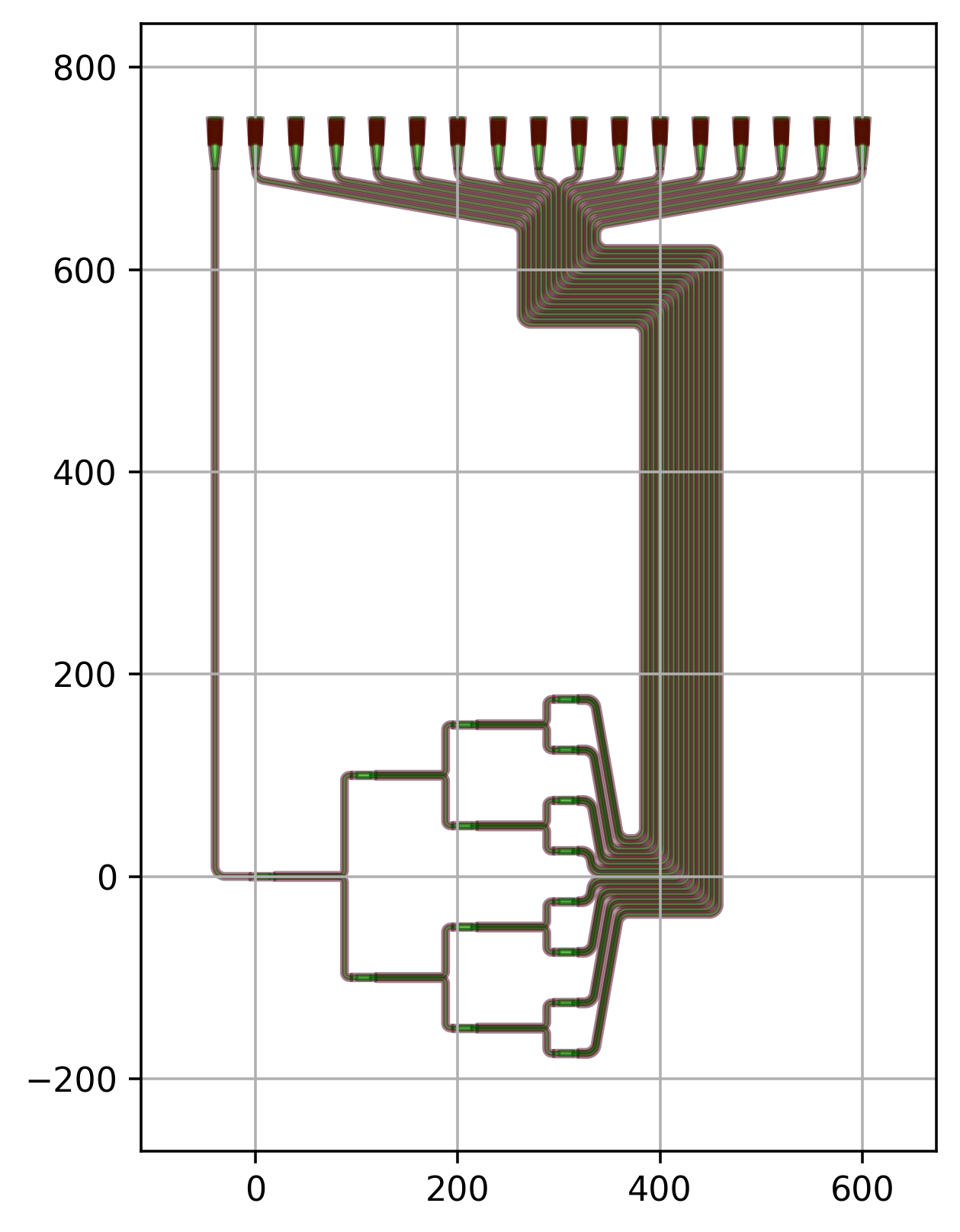
For example, consider a design with a splitter tree that needs to be connected to multiple grating couplers.

We want to create a bundle that consists of waveguides with a minimal bend radius of 10 µm, routed together as an array with a given pitch of 5 µm. Let’s start with a bundle with simple S-bend fanouts:
bend_radius = 10.0
pitch = 5.0
# Manhattan Bundle to connect the outputs of the splitter tree to the output grating couplers

bundle = [
    i3.ConnectManhattanBundle(
        connections=[(f"tree:out{16 - n}", f"gr_out_{n}:out") for n in range(16)],
        start_fanout=i3.SBendFanout(max_sbend_angle=80.0),
        end_fanout=i3.SBendFanout(max_sbend_angle=80.0),
        pitch=pitch,
        bend_radius=bend_radius,
    )
]
Here we specify the following parameters:
connections: It defines which port of the splitter tree is connected to which grating’s output port.start_fanoutandend_fanout: They specify the type of fanout used at the start and end of the bundle
In this case, we use i3.SBendFanout for the fanout.
This fanout can be customized by setting its properties, such as the pitch of the waveguide array, the max_sbend_angle the bend_radius, the min_spacing, etc.
The result looks as follows:
Bundle routing with obstacle avoidance
Routing a set of ports from one side of your design to another can be challenging, especially when there is limited space or the need to avoid other components. For instance, imagine there are other components in your design that the bundle needs to avoid.
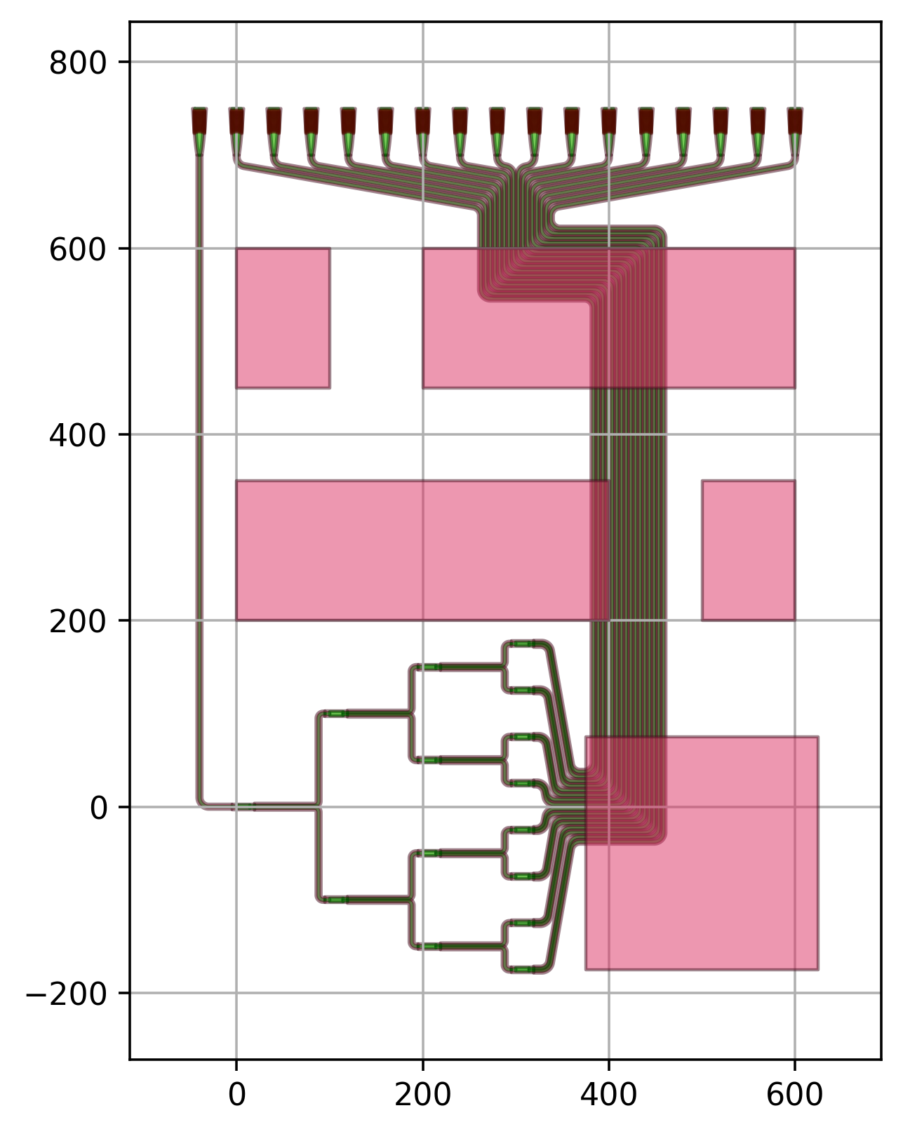
Similar to specifying control points in i3.ConnectManhattan, it is also possible to control the routing of a i3.ConnectManhattanBundle.
Let’s see how to do that, starting with the fanouts.
i3.ConnectManhattanBundle allows us to specify the start and the end fanouts independently:
start_fanout
This is the fanout at the output of the splitter tree.
Instead of having a symmetric fanout, the end needs to be shifted completely to the top.
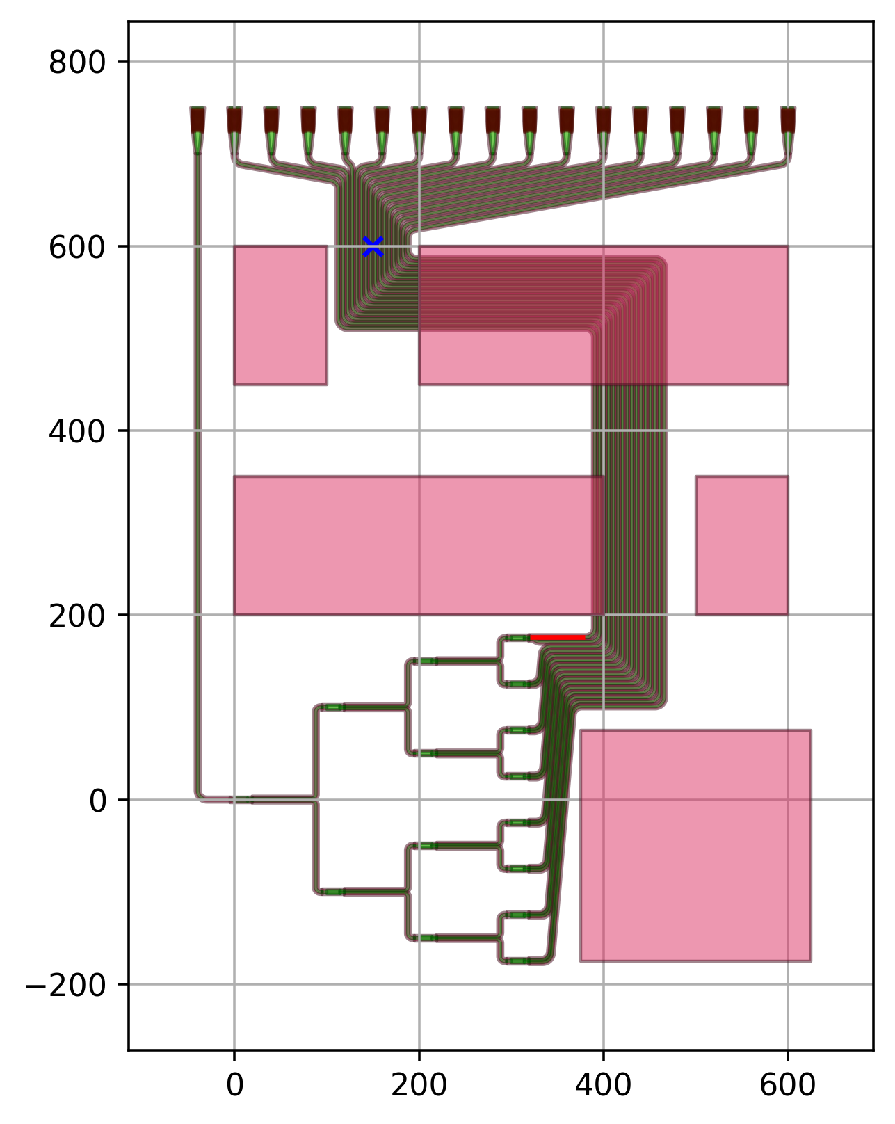
Ideally, the waveguide connected to the topmost port of the splitter tree (tree:out16) should go straight as indicated by the red line on the image below.
This can be achieved by defining the reference port.
This parameter determines which port the fanout should be aligned with.
If it isn’t defined, the center point of the input ports is used as the reference.
In addition, we need to tweak the max_sbend_angle parameter to increase the maximum angle the S-bends are allowed to make.
This ensures that the bundle is more compact and that the waveguides don’t overlap with the obstacle.
end_fanout
The center of the fanout needs to be between the two obstacles at the top.
Or rather, the end_position of the fanout needs to be at (150, 600) indicated by the blue cross on the image below.
bend_radius = 10.0
pitch = 5.0
# First, let's fix the fanouts

bundle = [
    i3.ConnectManhattanBundle(
        connections=[(f"tree:out{16 - n}", f"gr_out_{n}:out") for n in range(16)],
        start_fanout=i3.SBendFanout(max_sbend_angle=85.0, reference="tree:out16"),
        end_fanout=i3.SBendFanout(max_sbend_angle=80, end_position=(150, 600)),
        pitch=pitch,
        bend_radius=bend_radius,
    )
]
This results in the following.
Next, we need to adjust the routing of the waveguide bundle between the two fanouts.
Controlling the route of the Manhattan waveguide array can be done with horizontal and vertical control_points.
It is also possible to specify which waveguide of the bundle these control_points apply to.
The port that is connected to this waveguide should then be assigned as control_point_reference.
In order to define the control_points, some coordinates of one of our obstacles are used as anchors and then specified in i3.V and i3.H.
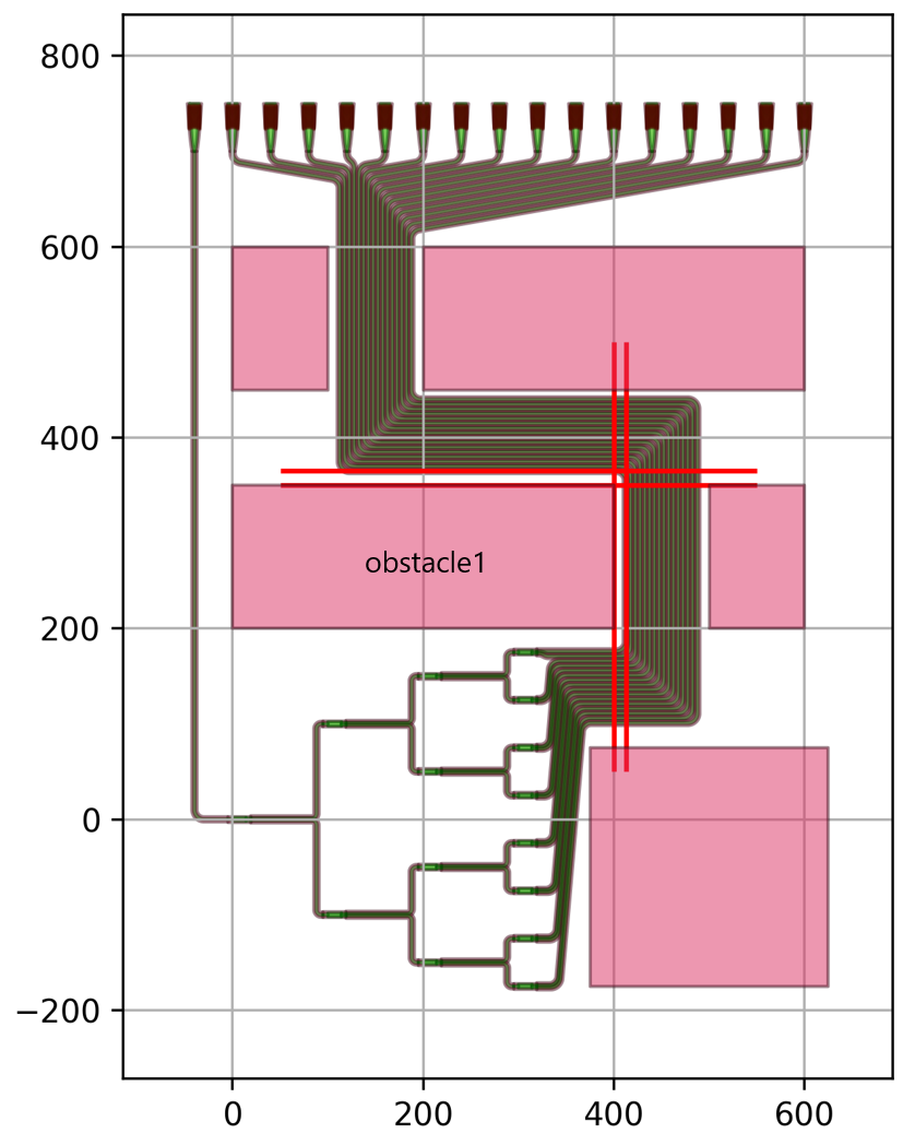
In this example below, we use the North and East coordinate of obstacle1, which is the first pink rectangle above the splitter tree.
The waveguide connected to the topmost port of the splitter (tree:out16) needs to first go vertically to the right of obstacle1 and then horizontally above obstacle1 as indicated by the vertical and horizontal lines in the image below.
# Next, the array of waveguides
# We use the properties control_point and control_point reference to adjust the routing

bundle = [
    i3.ConnectManhattanBundle(
        connections=[(f"tree:out{16 - n}", f"gr_out_{n}:out") for n in range(16)],
        start_fanout=i3.SBendFanout(max_sbend_angle=85.0, reference="tree:out16"),
        end_fanout=i3.SBendFanout(max_sbend_angle=80, end_position=(150, 600)),
        pitch=pitch,
        bend_radius=bend_radius,
        control_points=[i3.V(12.5, relative_to="obstacle1@E"), i3.H(15, relative_to="obstacle1@N")],
        control_point_reference="tree:out16",
    )
]
This results in the following:
Finally, by tweaking the bundle’s fanouts and array, we have obtained a bundle connector that carefully avoids obstacles.
Fully customized connection bundle
It is also possible to create a fully customized connection bundle by making use of a routing heuristic in your code. This approach offers you complete flexibility to program your own bundles in a parametric way. A few examples on how to create such a circuit is found in Addendum: Fully customized connection bundle.