Building a Parametric Model
In this section, we describe how to use Ansys Lumerical FDTD simulation data from a directional coupler PCell to build a parametric model. We then use this model to create an advanced directional coupler that allows you to specify the power fraction as an input parameter, instead of the coupling length. The model data is used to automatically determine the correct coupling length to achieve the desired input power fraction.
Note
This tutorial requires an installation of the Luceda Link for Ansys Lumerical. Please contact us for a trial license. For more detail on how to perform physical device simulation in Luceda IPKISS, please follow the Physical Device Simulation Flow tutorial, in particular the section on Ansys Lumerical FDTD.
Why Build a Parametric Model?
A parametric model allows designers to predict a component’s behavior across different layout configurations without running costly simulations for each variation. This is particularly useful for a directional coupler, where modeling performance at unsimulated straight lengths is essential for efficiently designing a PCell that takes a specific power fraction as input. Given the continuous nature of the parameter space, running countless simulations for every coupling length is both costly and time-consuming. Instead, we can run simulations for a limited number of coupling lengths and leverage advanced model-based interpolation to extract the directional coupler’s behavior at unsimulated coupling lengths. This enables you to specify a desired power fraction and use the interpolation coefficients to instantiate the directional coupler PCell with the correct straight length automatically.
IPKISS is the ideal tool for this, enabling parametric modeling through adjustable component parameters, automatic layout generation, and model-based interpolation all integrated into a streamlined design workflow.
Beyond efficiency, this approach provides flexibility. For instance, when designing a directional coupler for a different material platform, the same workflow can be reused to achieve a new optimized configuration and generate a new parametric model.
In this tutorial, we’ll systematically design a smart directional coupler by creating:
A DC PCell that serves as both the layout for simulation and the attachment point for the model.
A Simulation Recipe to simulate the electromagnetic behavior of the directional coupler, extract its scattering parameters (S-matrix), and generate data for building a compact model.
A Regeneration Function that consolidates all the necessary code to resimulate the directional coupler for a given set of parameters, fit the simulation data, and plot the results.
A Parametric Model for a directional coupler that is a function of wavelength and the straight length.
A Smart DC PCell that enables the user to define the desired specifications instead of physical parameters, using simulation data to determine the appropriate coupling length for a given power fraction.
In the following sections, we will focus on steps 3-5. For more information on steps 1-2, covering how the directional coupler layout is defined, the class hierarchy and simulation recipe, please refer to the next section Define a Directional Coupler PCell for Simulation.
Folder Structure
Before diving into the model-building process, it’s essential to first establish a clear and structured workflow. A well-organized project structure optimizes the design flow, improves collaboration, and ensures consistency across simulations, modeling, and layout generation.
In the SiFab demo PDK, the directional coupler folder follows a structured hierarchy:
si_fab
    ├── compactmodels
    └── components
        └── dir_coupler
            ├── data
            ├── doc
            ├── pcell
            ├── regeneration
            ├── simulation
            └── __init__.py
data: It contains the simulated, or measured, S-matrix data and the fitting parameters that are used to model the designed component when running circuit simulations.doc: It contains a documentation of the component, together with example scripts on how to use it.pcell: This is the core of the component. It contains the PCell definition and, if needed, other utilities used to design the component.regeneration: It contains a regeneration script to regenerate simulation data and fitting coefficients of the optimized component. This is useful to ensure the model data stored in thedatafolder is always up-to-date with the MMI layout.simulation: It contains the simulation recipe of the component.
By maintaining this structured approach, we ensure a clear separation of concerns, making it easier to iterate and validate designs efficiently.
The Regeneration and Fitting Step
In this section, we’ll implement a parametric model of our directional coupler by performing a polynomial fit of the simulated data from a layout. As mentioned, we’ll take a directional coupler PCell we have already designed and run simulations to build the model. An overview of the whole process is provided in the image below.
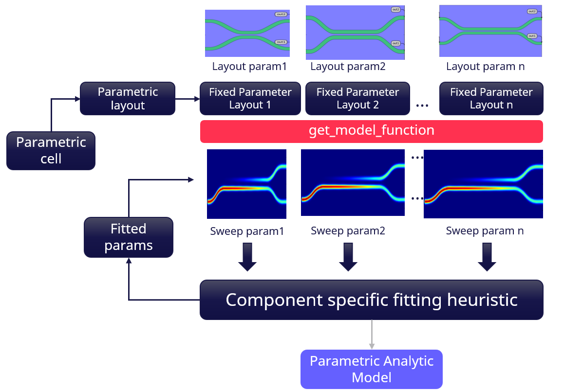
Let’s summarize the key steps.
Parametric Cell: Defines a layout where several parameters can be varied, such as material platform, waveguide shapes, or waveguide separation.
Layout Generation with Fixed Parameters: Layouts with fixed parameters are created by varying the coupling length.
Simulation & Model Extraction: Each fixed layout is simulated using Ansys Lumerical FDTD over a specified wavelength range
Component-Specific Fitting Heuristic: The simulation results are interpolated using a polynomial fitting heuristic to extract transmission and reflection coefficients as a function of coupling length and wavelength.
Parametric Model: The extracted parameters are used to build a parametric analytical model, enabling predictive behavior extraction without running new simulations.
To automate all these steps, we create a regeneration script. The goal is to:
Sweep over different lengths of the
SiDirectionalCouplerSPCell (available in the SiFab demo PDK) and save the data for each simulation in the data folder.Perform a polynomial fit of the simulation data to extract polynomial coefficients for transmission and reflection as a function of wavelength and straight length.
Store the polynomial coefficients in a file so that we can then use them when we build the circuit model.
As we have used a polynomial fitting, please note that this model will only be valid in the wavelength range that we have simulated (1.5 to 1.6 μm) and over a straight length range from 0 - 10 μm. Polynomial fitting is not ideal for data extrapolation outside of the simulated range.
The regeneration script is stored in the regeneration folder.
from si_fab import all as pdk  # noqa: F401
from regen_utils import regenerate_dc
from si_fab.components.dir_coupler.pcell.cell import SiDirectionalCouplerS
import numpy as np


regenerate_dc(
    dir_coupler_class=SiDirectionalCouplerS,
    lengths=np.linspace(0.0, 10.0, 11),
    wavelengths=(1.5, 1.6, 100),
    sim_sw="Lumerical",
    resimulate=True,
    refit=True,
    plot=True,
)
More details on how this fitting is performed can be found in the SiFab demo PDK at the following location: components/dir_coupler/regeneration/regen_utils.py.
Verifying the Model
An essential step in fitting a model is verifying its accuracy to ensure reliable predictions.
The regen_utils code contains functionality to evaluate the model by comparing simulated data from Lumerical with a polynomial fit across various lengths.
It produces plots showing power transmission and the normalized error to verify the accuracy of the model.
        # Creating the model data
        from si_fab.compactmodels.dir_coupler import get_transmission_kappa0_kappa

        smatrices = [
            convert_smatrix_units(
                i3.device_sim.SMatrix1DSweep.from_touchstone(
                    os.path.join(base_directory_sim, f"length{length}", "smatrix.s4p")
                ),
                to_unit="um",
            )
            for length in lengths
        ]
        wavelengths = smatrices[-1].sweep_parameter_values

        center_wavelength, pol_transmission, pol_kappa_0, pol_kappa = get_transmission_kappa0_kappa(
            wavelengths=wavelengths,
            smatrices=smatrices,
            lengths=lengths,
            deg=3,
            plot=plot,
        )

        results_np = {
            "center_wavelength": center_wavelength,
            "pol_transmission": pol_transmission,
            "pol_kappa_0": pol_kappa_0,
            "pol_kappa": pol_kappa,
        }

        def serialize_ndarray(obj):
            return obj.tolist() if isinstance(obj, np.ndarray) else obj

        params_path = os.path.join(base_directory_model, "params.json")

        with open(params_path, "w") as f:
            json.dump(results_np, f, sort_keys=True, default=serialize_ndarray, indent=2)

    # Plots
    if plot:
        for S, length in zip(smatrices, lengths):
            dc = dir_coupler_class(name=f"_{length}", straight_length=length)
            dc_cm = dc.CircuitModel()
            Smodel = dc_cm.get_smatrix(wavelengths=wavelengths)

            plt.plot(wavelengths, i3.signal_power(S["out1", "in1"]), label=f"through_{length}_sim")
            plt.plot(wavelengths, i3.signal_power(S["out2", "in1"]), label=f"drop_{length}_sim")
            plt.plot(wavelengths, i3.signal_power(Smodel["out1", "in1"]), "*", label=f"through_{length}_fit")
            plt.plot(wavelengths, i3.signal_power(Smodel["out2", "in1"]), "*", label=f"drop_{length}_fit")
            plt.xlabel("Wavelength [um]")
            plt.ylabel("Power [dB]")
            plt.legend()
            plt.show()

        for S, length in zip(smatrices, lengths):
            dc = dir_coupler_class(name=f"_{length}", straight_length=length)
            dc_cm = dc.CircuitModel()
            Smodel = dc_cm.get_smatrix(wavelengths=wavelengths)

            tot_power = i3.signal_power(S["out2", "in1"]) + i3.signal_power(S["out1", "in1"])
            error_through = (i3.signal_power(S["out1", "in1"]) - i3.signal_power(Smodel["out1", "in1"])) / tot_power
            error_cross = (i3.signal_power(S["in1", "out2"]) - i3.signal_power(Smodel["in1", "out2"])) / tot_power

            plt.plot(wavelengths, error_through, label=f"error_through_{length}")
            plt.plot(wavelengths, error_cross, label=f"error_cross_{length}")

        plt.xlabel("Wavelength [um]")
        plt.ylabel("Normalized error")
        plt.legend()
        plt.show()
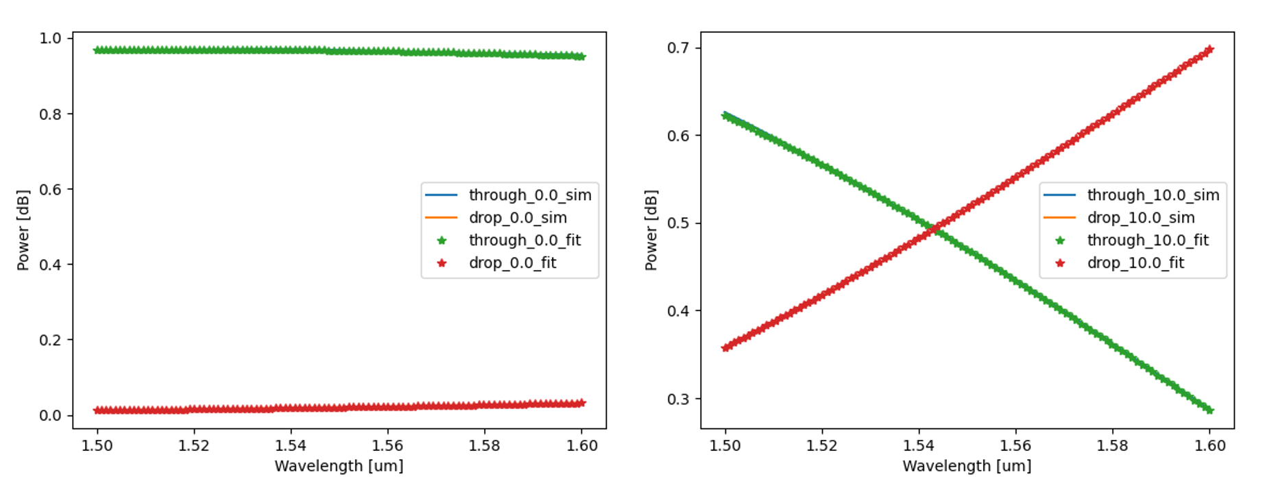
After executing the regeneration script for the S-shaped directional coupler we can inspect the performance and model accuracy. The three plots below show how the directional coupler performs across the coupling lengths and wavelengths given as inputs, while also demonstrating the accuracy of the model fit.
First Plot: When the coupling length is 0.0 μm, nearly all the light stays in the through port (power close to 0 dB), and almost none reaches the drop port. This makes sense since there’s no interaction length for coupling to occur. At a coupling length of 10.0 μm around 1540 nm, the power splits evenly between the through and drop ports (both at about -3 dB).
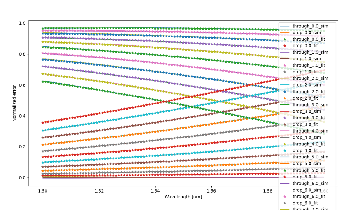
Second Plot: Combines data from 11 simulated straight lengths and shows how accurately our fitted model interpolates across the full range of lengths and wavelengths. It gives a clear picture of both the directional coupler’s performance and the model’s reliability.
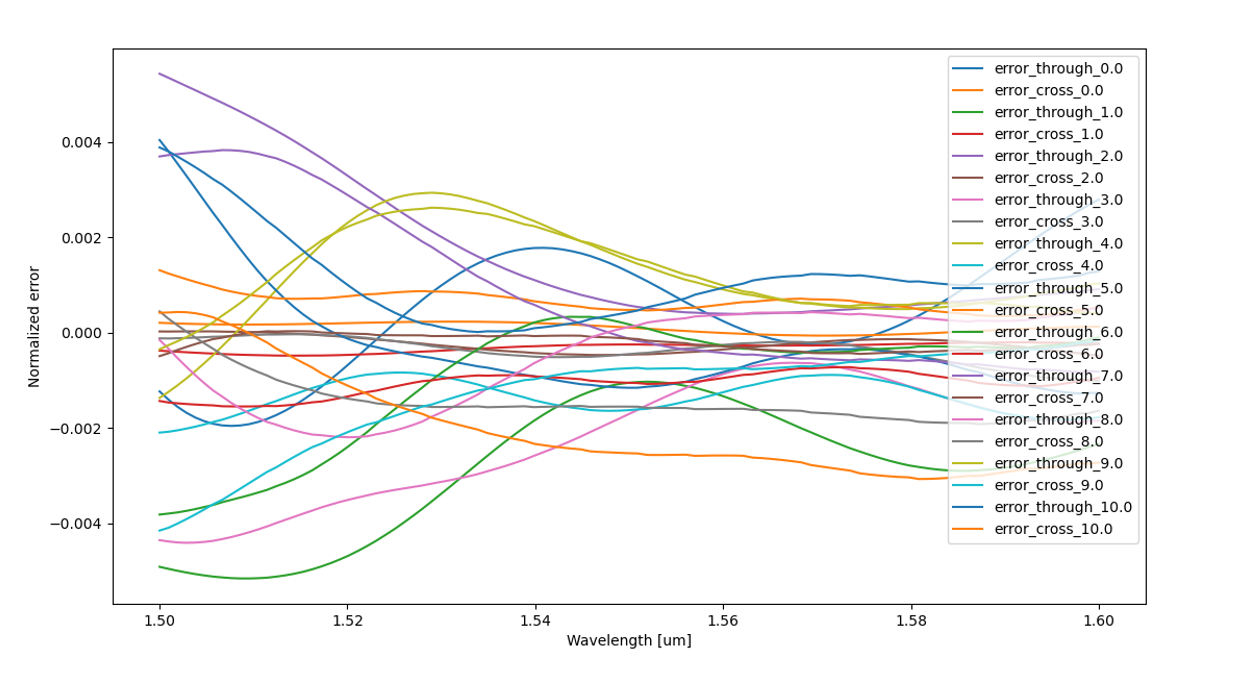
Third Plot: Shows the normalized error across the coupling lengths 0.0 to 10.0 μm and the wavelength range 1.5 to 1.6 μm. We verify the precision by noting the differences between the simulated and fitted results are within ±0.002 with a slight increase (±0.004) at the edges of the wavelength range.
50:50 Directional Coupler at 1550 nm
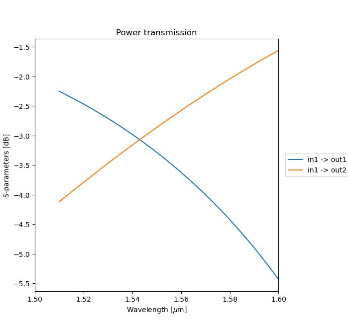
Let’s now instantiate the directional coupler at a specific coupling length and visualize the circuit simulation, which uses the polynomial fit of the FDTD simulation data. We see that a straight length of 10 μm results in a near 50:50 split at around 1.54 μm.
from si_fab import all as pdk
import numpy as np

dc = pdk.SiDirectionalCouplerS(straight_length=10.0)
dc_lv = dc.Layout()
dc_lv.visualize(annotate=True)

dc_cm = dc.CircuitModel()

wavelengths = np.linspace(1.51, 1.6, 500)
S = dc_cm.get_smatrix(wavelengths=wavelengths)
S.visualize(
    term_pairs=[
        ("in1", "out1"),  # through
        ("in1", "out2"),  # drop
    ],
    scale="dB",
    title="Power transmission",
    xrange=(1.5, 1.6),
If we wanted to instantiate a directional coupler with a perfect 50:50 split at our desired target wavelength of 1.5 μm using the SiDirectionalCouplerS PCell, we would need to repeat this process by gradually varying the coupling length, until we reach the desired transmission spectrum.
To accelerate and automate this process, we can leverage the power of parametric modeling.
We design a directional coupler that accepts any power fraction in the range of 0 to 1 at a target wavelength as an input parameter, using the fitting data to automatically calculate the correct coupling length to achieve the desired power fraction.
To do this, we create a new PCell SiDirectionalCouplerSPower that adjusts its coupling length based on the fitted model.
The coupling length is computed dynamically using the data obtained from simulation inside the get_length_from_power_fraction function.
def get_length_from_power_fraction(power_fraction, pol_kappa, pol_kappa0, target_wavelength, center_wavelength):
    """Calculate the length of a directional coupler required to obtain a given coupled power ratio in the cross arm.

    Parameters
    ----------
    power_fraction : float
        Fraction of output power coupled into the cross arm. Losses are considered. Valued allowed between 0 and 1
    pol_kappa : list of coefficients of the polynomial fit of kappa as function of wavelength
    pol_kappa0 : list of coefficients of the polynomial fit of kappa0 as function of wavelength
    target_wavelength : float
        Target wavelength in um
    center_wavelength : float
        Center wavelength of the polynomial fit in um
    length : float
        Length of the directional coupler with power ratio in the cross arm given by power_fraction. The value of the
        length is snapped to the grid

    Returns
    --------
    length : float
        Length corresponding to the specified power fraction
    """

    if power_fraction > 1 or power_fraction < 0:
        raise ValueError("power_coupling has to be between 0 and 1")

    kappa = np.polyval(pol_kappa, target_wavelength - center_wavelength)
    kappa0 = np.polyval(pol_kappa0, target_wavelength - center_wavelength)
    power_field = np.sqrt(power_fraction)

    cnt = np.ceil((kappa0 - np.arcsin(power_field)) / (2 * np.pi))
    length = (np.arcsin(power_field) - kappa0 + 2 * np.pi * cnt) / kappa
In get_length_from_power_fraction function, we ensure that the power fraction is within the valid range of 0 to 1 as values outside this range would be physically impossible.
Next, we use polynomial models (pol_kappa and pol_kappa0) to determine the coupling coefficients at the target wavelength.
Since power transfer in a directional coupler follows sinusoidal behavior, we convert the power fraction to its corresponding field amplitude and use trigonometric functions to compute the phase-matching condition.
To ensure the correct coupling occurs, we adjust for phase periodicity using a 2π multiple.
Now we have a directional coupler PCell with a parametric model to create our 50:50 power coupling.
In the doc folder, we create a script to simulate the parametric layout, which takes power fraction and target wavelength as inputs and plots the results.
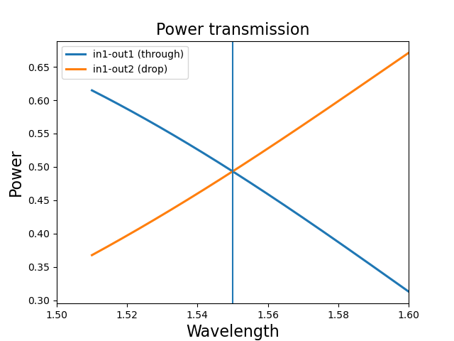
We can now easily instantiate the directional coupler with perfect 50:50 split at 1.5 μm wavelength by running this script only once.
dc = pdk.SiDirectionalCouplerSPower(power_fraction=0.5, target_wavelength=1.55)
dc_lv = dc.Layout()
dc_lv.visualize(annotate=True)

dc_cm = dc.CircuitModel()

wavelengths = np.linspace(1.51, 1.6, 500)
S = dc_cm.get_smatrix(wavelengths=wavelengths)
S.visualize(term_pairs=[("in1", "out1"), ("in1", "out2")], title="Transmission")
Conclusion
In this section of the tutorial, we developed a parametric model for a silicon directional coupler, enabling design based on a target power fraction. By leveraging simulation data, we extracted key parameters and applied polynomial fitting to accurately model the coupler’s behavior across a range of wavelengths and coupling lengths.
This model allows designers to specify a desired power fraction at a target wavelength and instantly determine the corresponding coupling length, eliminating the need for additional simulations. The ability to automate this process is further enhanced by the regeneration script, which streamlines data extraction, fitting, and model integration into a locked PCell.
The result is a flexible, simulation-driven approach that accelerates the prototyping and optimization of directional couplers. With this methodology, designers can efficiently create directional couplers with any power fraction.
Note
To learn more about how to define the directional coupler PCells, please read the next section.