WG3

class ipkiss3.cml.WG3

Single mode polynomial waveguide model.

Uses a polynomial expression of the effective index and loss (in dB/m) as function of wavelength and temperature offset .

Parameters:

n_eff: List[List[float]]

Polynomial coefficients of the mode effective index as function of wavelength and temperature offset. First row contains the highest order wavelength-dependent terms, while the last row contains wavelength-independent terms. Similarly, the first column contains the highest order temperature-dependent terms, while the last column contains temperature-independent terms.

loss: List[float]

Polynomial coefficients [dB/um / (um)^n] of the loss of the waveguide mode as function of wavelength offset from center_wavelength. Highest order first (loss at center_wavelength last).

center_wavelength: float (um)

Center wavelength (in micrometer) of the model around which n_eff and loss are defined.

center_temperature: float (au)

Center temperature (in arbitrary units) of the model around which n_eff is defined.

length: float (um)

Total length of the waveguide in micrometer.

Notes

The effective index is calculated as:

$$n_{eff}(\lambda ,T)=\sum _{i=0}^M\sum _{j=0}^N{n}_{eff}[i,j](\lambda -{\lambda }_c{)}^{M-i}(T-T_c{)}^{N-j}$$

Where M and N represent the order of the polynomial in terms of wavelength and temperature, respectively. ${\lambda }_c$ is the central wavelength and $T_c$ is the central temperature.

Similarly, the loss is defined as

$$loss(\lambda )=\sum _{i=0}^{P}loss[i](\lambda -{\lambda }_c{)}^{P-i}$$

Note

All wavelengths, including those in the polynomial expansions, are represented in micrometers.

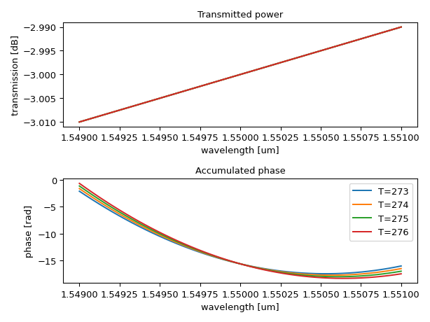
Frequency domain

The scatter matrix is given by:

$$\begin{array}{r}{\mathbf{S}}_{wg}=\left[\begin{array}{cc}0& \exp (-j\frac{2\pi }{\lambda }L{n}_{eff}(\lambda ,T))\ast A\\ \exp (-j\frac{2\pi }{\lambda }L{n}_{eff}(\lambda ,T))\ast A& 0\end{array}\right]\end{array}$$

Where the amplitude loss is calculated as:

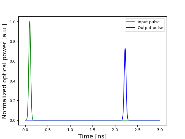
$$A={10}^{-loss\ast L/20.0}$$

Time domain

The electric field at the output is

$$E_{out}(\lambda ,T)=\exp (j{\varphi }_0)E_{in}(t-L{n}_g(\lambda ,T)/c)\ast A$$

where the group index is derived from the effective index by

$$n_g(\lambda ,T)=n_{eff}(\lambda ,T)-\lambda \frac{d}{d\lambda }{n}_{eff}(\lambda ,T)$$

Terms

Term Name	Type	#modes
in	Optical	1
out	Optical	1

Examples

import ipkiss3.all as i3
import matplotlib.pyplot as plt
import numpy as np

class CustomWaveguide(i3.Waveguide):
    class CircuitModel(i3.CircuitModelView):
        def _generate_model(self):
            # Model effective index assuming there is a linear dependence on both wavelength and temperature
            # neff = n0 + wl_coeff * dwl + thermal_coeff * dT
            n0 = 2.57
            wl_coeff = -0.85  # First order wavelength dependence
            thermal_coeff = 1.86 * 10**-4  # First order temperature dependence (thermo-optic coefficient)
            return i3.cml.WG3(
                n_eff=[
                    [0, wl_coeff],
                    [thermal_coeff, n0],
                ],
                loss=[-10.0 * 1e-6, 3.0 * 1e-6],
                center_wavelength=1.55,
                center_temperature=273,
                length=1e6,
            )

wavelengths = np.linspace(1.549, 1.551, 50)
temperatures = [273, 274, 275, 276]
cm = CustomWaveguide().CircuitModel()
s_matrices = [cm.get_smatrix(wavelengths, temp, debug=True) for temp in temperatures]

plt.subplot(211)
plt.xlabel("wavelength [um]")
plt.ylabel("transmission [dB]")
plt.title("Transmitted power")
for S, temp in zip(s_matrices, temperatures):
    transmission = 10 * np.log10(np.abs(S["out", "in"]) ** 2)
    plt.plot(wavelengths, transmission, label=f"T={temp}")

plt.subplot(212)
plt.xlabel("wavelength [um]")
plt.ylabel("phase [rad]")
plt.title("Accumulated phase")
for S, temp in zip(s_matrices, temperatures):
    phase = np.unwrap(np.angle(S["out", "in"]))
    plt.plot(wavelengths, phase, label=f"T={temp}")
plt.tight_layout()
plt.legend()
plt.show()

import ipkiss3.all as i3
import numpy as np
import matplotlib.pyplot as plt

class CustomWaveguide(i3.Waveguide):
    class CircuitModel(i3.CircuitModelView):
        def _generate_model(self):
            n0 = 2.57
            wl_coeff = -0.85
            thermal_coeff = 1.86 * 10**-4  # thermo-optic coefficient
            return i3.cml.WG3(
                n_eff=[
                    [0, wl_coeff],
                    [thermal_coeff, n0],
                ],
                loss=[-10.0 * 1e-6, 5.0 * 1e-6],
                center_wavelength=1.55,
                center_temperature=273,
                length=0.25 * 1e6,
            )

def optical_pulse(optical_power=1.0, t_offset=1e-11, pulse_width=1e-9):
    """Create an optical pulse"""

    def f_pulse(t):
        sigma = pulse_width / (2.0 * np.sqrt(2.0 * np.log(2.0)))
        return np.sqrt(optical_power * np.exp(-(((t - t_offset) / (np.sqrt(2.0) * sigma)) ** 2)))

    return f_pulse

opt_pulse_source = i3.FunctionExcitation(
    port_domain=i3.OpticalDomain,
    excitation_function=optical_pulse(optical_power=1.0, t_offset=1e-10, pulse_width=5e-11),
)

testbench = i3.ConnectComponents(
    child_cells={
        "opt_in": opt_pulse_source,
        "wg": CustomWaveguide(),
        "opt_out": i3.Probe(port_domain=i3.OpticalDomain),
    },
    links=[
        ("opt_in:out", "wg:in"),
        ("wg:out", "opt_out:in"),
    ],
)

# Simulation
sim_result = testbench.CircuitModel().get_time_response(
    t0=0.0, t1=3e-9, dt=0.5e-12, center_wavelength=1.50, temperature=270, debug=True
)
time_data = sim_result.timesteps
input_power = np.abs(sim_result["opt_in"]) ** 2
output_power = np.abs(sim_result["opt_out"]) ** 2

# Plot the results
plt.plot(time_data * 1e9, input_power, "g-", label="Input pulse")
plt.plot(time_data * 1e9, output_power, "b-", label="Output pulse")
plt.xlabel(r"Time [ns]", fontsize=15)
plt.ylabel(r"Normalized optical power [a.u.]", fontsize=15)
plt.legend()
plt.show()