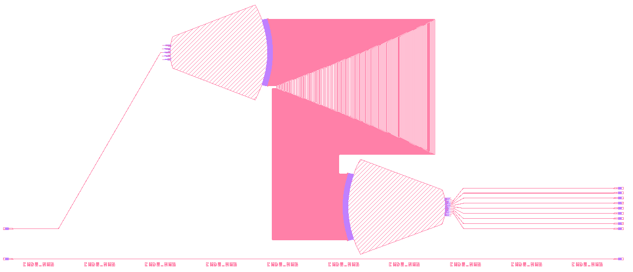
Organizing your AWG design project
In this application example, you will learn how to use Luceda AWG Designer to organize a project for designing an AWG. The target application of our AWG is one for IEEE 400Gb Ethernet [1] standard 400GBase-LR8 [2]. We will consider a situation in which we are developing such an AWG and want to tape out test designs of the AWG to a foundry to test it. We will take the script for an AWG that we developed in the tutorial on Getting Started with AWG Designer and organize it into different functions so that it can be iterated upon and prepared for tape-out.
As an exercise, you will also learn how to change the parameters of your AWG and see how its performance varies, taking into account design trade-offs.
Organize your code in different files
Once you have created your code for designing your AWG, we recommend that you organize it into different functions that can be easily maintained. In this example, we have the following:
generate_awg: it executes all the steps for the AWG generation and it returns an AWG PCell.simulate_awg: it takes the generated AWG PCell as an input, simulates it and returns its S-matrix.analyze_awg: it takes an S-matrix as an input, performs the analysis and returns a report on the specifications.finalize_awg: it takes an AWG PCell as an input and returns a routed and fab-ready AWG in GDSII format.
While you iterate on your designs, you would be able to customize them and choose the desired parameters that need to be varied.
Then, you would have a master script that goes through all these functions.
In this example, we use the code below.
It goes through all the steps and stores the results in the folder designs/awg_10400_0.4, which contains:
The finalized GDSII file of the AWG
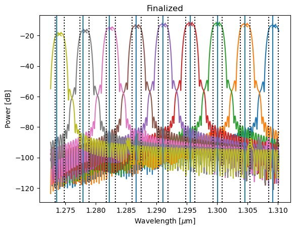
The simulated spectrum
An analysis report
import si_fab.all as pdk  # noqa: F401
import ipkiss3.all as i3
import numpy as np
import os

from rect_awg.generate import generate_awg
from rect_awg.simulate import simulate_awg
from rect_awg.finalize import finalize_awg
from rect_awg.analyze import analyze_awg

# Actions
generate = True
simulate = True
analyze = True
finalize = True
plot = True

# Specifications
wg_width = 0.4
fsr = 10400

# Creating a folder for results
this_dir = os.path.abspath(os.path.dirname(__file__))
designs_dir = os.path.join(this_dir, "designs")
if not os.path.exists(designs_dir):
    os.mkdir(designs_dir)
save_dir = os.path.join(designs_dir, f"awg_{fsr}_{wg_width:.1f}")
if not os.path.exists(save_dir):
    os.mkdir(save_dir)

# Simulation specs
wavelengths = np.linspace(1.26, 1.32, 1000)

# Bare AWG
if generate:
    awg = generate_awg(fsr=fsr, wg_width=wg_width, plot=plot, save_dir=save_dir, tag="bare")
if simulate:
    smat = simulate_awg(awg=awg, wavelengths=wavelengths, save_dir=save_dir, tag="bare")
else:
    path = os.path.join(save_dir, "smatrix_bare.s10p")
    smat = i3.device_sim.SMatrix1DSweep.from_touchstone(path, unit="um") if os.path.exists(path) else None

if analyze:
    analyze_awg(smat, plot=True, save_dir=save_dir, tag="bare")

# Finished AWG
if finalize:
    if generate:
        finalized_awg = finalize_awg(awg=awg, plot=plot, save_dir=save_dir, tag="finalized")

    if simulate:
        smat_finalized = simulate_awg(
            awg=finalized_awg.blocks[3],
            wavelengths=wavelengths,
            save_dir=save_dir,
            tag="finalized",
        )
    else:
        path = os.path.join(save_dir, "smatrix_finalized.s10p")
        smat_finalized = i3.device_sim.SMatrix1DSweep.from_touchstone(path, unit="um") if os.path.exists(path) else None

    if analyze:
        analyze_awg(smat_finalized, peak_threshold=-25, plot=plot, save_dir=save_dir, tag="finalized")

print("Done")


Analysis report: report_finalized.json
Let’s now take a look at generate_awg.
As explained above, it executes all the steps for the AWG generation and returns an AWG PCell.
In this project this function is defined in rect_awg/generate.py.
Let’s have a look at the function signature.
def generate_awg(fsr, wg_width=0.4, plot=True, save_dir=None, tag=""):
    """Custom AWG generating function. If you make an AWG, you should write one of your own.
    Parameters are the things you want to vary as well as options to control if you
    plot and where you save your data.

    Parameters
    ----------
    fsr : float
          FSR of the AWG in Hz
    wg_width : float, default: 0.4, optional
               Width of the waveguides in the array
    plot : bool, default: True, optional
           If true the AWG is plotted
    save_dir: str, default: None, optional
              If specified, a GDSII file is saved in this directory
    tag: str, optional
         String used to give a name to saved files

    Returns
    -------
    cwdm_awg : i3.PCell
               AWG PCell
    """

    center_frequency = 232200.0  # GHz
    n_channels = 9
    channel_spacing = 800.0  # GHz
As you can see, fsr and wg_width are provided as parameters that you can vary. These parameters are passed to the design function and to the waveguide template, respectively. These allow us to vary both of these parameters in our design in order to see how they affect it.
In your own AWG designs, you can define which parameters you want to expose.
The function generate_awg goes through all the steps of instantiating the AWG components, synthesising the AWG and assembling it that are detailed in the sections on synthesis and assembly of the tutorial on getting started with AWG Designer.
The code is the same, it is simply restructured and wrapped into this function.
It then returns an AWG PCell with the layout obtained by assembling the AWG.
Similarly, the functions simulate_awg and analyze_awg use the same code as in the section on simulation and analysis of that tutorial and wraps around them for usability.
The former takes the AWG PCell and a set of wavelengths as input and returns the simulated S-matrix.
from ipkiss3 import all as i3
import os


def simulate_awg(awg, wavelengths, save_dir=None, tag=""):
    """Custom function to simulate an AWG. If you make an AWG, you should write one of your own.
    Parameters are the awg cell you want to simulate and things that control your simulation as well as
    parameters that control where you save your data.

    Parameters
    ----------
    awg : i3.Pcell
          AWG PCell
    wavelengths: ndarray
                 Simulation wavelengths
    save_dir: str, default: None, optional
              If specified, a GDSII file is saved in this directory
    tag: str, optional
         String used to give a name to saved files

    Returns
    -------
    awg_s:
           S-matrix of the simulated AWG

    """
    cwdm_awg_cm = awg.get_default_view(i3.CircuitModelView)
    print("Simulating AWG...\n")
    awg_s = cwdm_awg_cm.get_smatrix(wavelengths)
    if save_dir:
        smatrix_path = os.path.join(save_dir, f"smatrix_{tag}.s{awg_s.data.shape[0]}p")
        awg_s.to_touchstone(smatrix_path)
        print(f"{smatrix_path} written")
    return awg_s
Whereas the latter takes the simulated s-matrix together with other optional parameters you can define (see the signature below), prints out an analysis report and displays the result of the simulation and and channel locations in a figure.
def analyze_awg(awg_s, peak_threshold=-10.0, plot=True, save_dir=None, tag=""):
    """Custom AWG analysis function. If you make an AWG, you should write an analysis function of your own.
    The goal of the analyze_awg function is to answer the question: how does the AWG perform
    according to my specs? In an analysis function you define the specs and check the behaviour
    of the AWG according to those specs using helper functions provided in the Luceda AWG Designer.
    The parameters are the things you want to vary as well as options to control whether you
    plot and where you save your data.

    Parameters
    ----------
    awg_s: SMatrix1DSweep
        S-matrix of the AWG
    peak_threshold: float, default: -10.0, optional
        The power threshold for peak detection (in dB)
    plot: bool, default: True, optional
        If true, the spectrum is plotted
    save_dir: str, default: None, optional
        If specified, a GDSII file is saved in this directory
    tag: str, optional
        String used to give a name to saved files

    Returns
    ------
    report: dict
        Dictionary containing analysis specs
    """
The only function with code that is substantially changed from the tutorial on Getting Started with Luceda AWG Designer is finalize_awg, whose function signature is shown below.
def finalize_awg(awg, plot=True, die_width=3000.0, save_dir=None, tag=""):
    """Custom function to finalize an AWG design, mostly for DRC fixing and routing.
    If you make an AWG, you should write one of your own.
    Parameters are the things you want to vary as well as options to control whether you
    plot and where you save your data.

    Parameters
    ----------
    awg: i3.PCell
         Input AWG cell
    plot : bool, default: True, optional
           If true the finilized awg is plotted
    die_width: float, default: 3000.0, optional
               Width of the die
    save_dir : str, default: None, optional
               If specified, a GDSII file is saved in this directory
    tag: str, optional
         String used to give a name to saved files

    Returns
    -------
    awg_block: i3.PCell
               Finalized AWG block
    """
It takes an AWG PCell as input together with whichever optional parameters you want, fixes common DRC errors, and includes it in a small test design that can be merged in a top-level layout as explained in the finalization step of that tutorial.
Final simulation and analysis
Now we can simulate the transmission of the devices on the chip to check that our test structures allow us to extract the information we need about the device under test (the AWG in this case).
As you may recall in the tutorial on the finalization step, the alignment waveguide is the second object we added to the block (index 1) and the AWG is the fourth (index 3).
We retrieve their circuit models from which we simulate the spectra.
All effects in the devices under test are taken into account, including the waveguide losses and the performance of the fiber grating couplers.
In addition, we can use the previously defined simulate_awg and analyze_awg functions to analyze the S-matrix of the AWG, including the behavior from the fiber grating couplers.
Since the transmitted power has considerably dropped due to the fiber grating couplers, we set the threshold for peak detection to -25 dB.
# Finished AWG
if finalize:
    if generate:
        finalized_awg = finalize_awg(awg=awg, plot=plot, save_dir=save_dir, tag="finalized")

    if simulate:
        smat_finalized = simulate_awg(
            awg=finalized_awg.blocks[3],
            wavelengths=wavelengths,
            save_dir=save_dir,
            tag="finalized",
        )
    else:
        path = os.path.join(save_dir, "smatrix_finalized.s10p")
        smat_finalized = i3.device_sim.SMatrix1DSweep.from_touchstone(path, unit="um") if os.path.exists(path) else None

    if analyze:
        analyze_awg(smat_finalized, peak_threshold=-25, plot=plot, save_dir=save_dir, tag="finalized")

print("Done")

Report JSON file: report_finalized.json
We can clearly see the fiber coupler spectrum overlayed (twice, for the input and the output coupler) on the alignment waveguide and the AWG. The spectrum of the AWG test structure can then be normalized to the one of the alignment waveguide to get a relatively accurate estimate of the transmission of the AWG itself.
Conclusion
In this tutorial, we have organized code for designing an AWG so that it matches well the four design steps:
AWG generation
AWG simulation
AWG analysis
AWG finalization
We have made sure that the AWG adheres to layout design rules, and we’ve routed the AWG to the outside world to obtain a design ready for tape-out. Finally, a test structure was created and validated in simulation for testing and extracting the AWG performance.
Test your knowledge
In order to become familiar with the procedure for maintaining and iterating your designs, please run the following file:
luceda-academy/training/topical_training/organize_awg_project/example_generate_awg.py
As an exercise, try to change the FSR of the AWG to 12000 GHz and compare the result with the 10400 GHz.
Has the insertion loss increased or decreased?
Has the crosstalk increased or decreased?
You can try creating a parameter sweep using a for loop.