camfr_guided_modes

ipkiss3.all.device_sim.camfr_guided_modes(material_stack, wavelengths, pml_thickness=0.0)

Calculates the neff for guided modes for a material stack using the camfr mode solver.

Parameters:

material_stack: MaterialStack object

The stack of ipkiss materials to calculate the modes for.

wavelengths: array_like

An array of wavelengths to calculate the modes for.

pml_thickness: float

Thickness of the complex Perfectly Matched Layer to use.

Returns:

guided_modes: dict

Returns a dictionary that maps the mode names onto a numpy array that contains the wavelength and the corresponding mode effective index.

Examples

import si_fab.all as pdk
from ipkiss.technology import get_technology
TECH = get_technology()
import ipkiss3.all as i3
import numpy as np
import matplotlib.pyplot as plt
from pysics.basics.material.material_stack import MaterialStack

# we define a MaterialStack
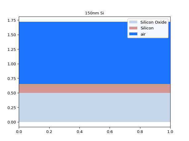
mstack = MaterialStack(
    name="150nm Si",
    materials_heights=[
       (TECH.MATERIALS.SILICON_OXIDE, 0.500),
       (TECH.MATERIALS.SILICON, 0.150),
       (TECH.MATERIALS.AIR, 1.070)
   ]
)

# use the MaterialStack method to plot it
mstack.visualize()

wavelengths = np.linspace(1.54, 1.56, 10)
neffs = i3.device_sim.camfr_guided_modes(mstack, wavelengths)

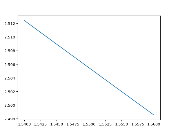
# Now we plot the zeroth-order mode:
TE0 = neffs['TE0']

# TEO is 'structured numpy array', this means it has fields
# in this case it has a wavelength and n_eff field.

wls = TE0['wavelength']
# n_eff is a complex number
neffs = TE0['n_eff'].real

plt.plot(wls, neffs)
plt.show()

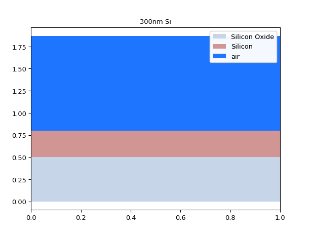
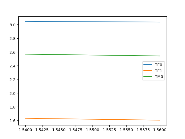
# If we make the core higher
# we should see higher order modes appear
mstack = MaterialStack(
    name="300nm Si",
    materials_heights=[
       (TECH.MATERIALS.SILICON_OXIDE, 0.500),
       (TECH.MATERIALS.SILICON, 0.300),
       (TECH.MATERIALS.AIR, 1.070)
   ]
)

mstack.visualize()

results = i3.device_sim.camfr_guided_modes(mstack, wavelengths)

for mode_name, neffs in results.items():
    plt.plot(neffs['wavelength'], neffs['n_eff'].real, label=mode_name)
plt.legend(results.keys())
plt.show()

Sometimes you’ll want to write/load the data to/from a file. To allow reading it from a different application or just to avoid running the simulation multiple times.

# With Python's builtin pickle module it's easy to write
# and load the data to/from a data file.

import si_fab.all as pdk
from ipkiss.technology import get_technology
TECH = get_technology()
from pysics.basics.material.material_stack import MaterialStack
import ipkiss3.all as i3
import numpy as np

mstack = MaterialStack(
    name="300nm Si",
    materials_heights=[
        (TECH.MATERIALS.SILICON_OXIDE, 0.500),
        (TECH.MATERIALS.SILICON, 0.300),
        (TECH.MATERIALS.AIR, 1.070)
    ]
)

wavelengths = np.linspace(1.54, 1.56, 10)
results = i3.device_sim.camfr_guided_modes(mstack, wavelengths)

# to write to the file
import pickle

with open('out.dat', 'wb') as out:
    pickle.dump(results, out)

fin = open('out.dat', 'rb')
results_new = pickle.load(fin)
fin.close()

# in case you want to export to a textual format, e.g a csv file
# you can use np.savetxt, though this requires a bit more work:

def savetocsv(filename, results):
    results_items = results.items()
    data = np.hstack([val for _, val in results_items])
    dtype = [
        ('mode_name', 'S10'),
        ('wavelength', np.float64),
        ('neff_real', np.float64),
        ('neff_imag', np.float64)
    ]

    results_np = np.zeros(
        len(data),
        dtype=dtype
    )

    offset = 0
    for mode_name, result in results_items:
        results_np['mode_name'][offset:offset + len(result)] = mode_name
        offset += len(result)

    results_np['wavelength'] = data['wavelength']
    results_np['neff_real'] = data['n_eff'].real
    results_np['neff_imag'] = data['n_eff'].imag

    np.savetxt(filename, results_np, delimiter=',', fmt=['%s', '%.18e', '%.18e', '%.18e'])

savetocsv('guided_modes.csv', results)

# to load the csv data again, you can use np.loadtxt:

def loadfromcsv(filename):
    # we assume the same order as used in the savetocsv
    dtype = [
        ('mode_name', 'S10'),
        ('wavelength', np.float64),
        ('neff_real', np.float64),
        ('neff_imag', np.float64)
    ]

    raw_data = np.loadtxt(filename, dtype=dtype, delimiter=',')
    mode_names = np.unique(raw_data['mode_name']).tolist()
    results = {}

    for mode_name in mode_names:
        mask = raw_data['mode_name'] == mode_name
        mode_data = raw_data[mask][['wavelength', 'neff_real', 'neff_imag']]
        results[mode_name] = np.rec.fromarrays(
            [mode_data['wavelength'], mode_data['neff_real'] + 1j * mode_data['neff_imag']],
            names='wavelength, n_eff'
        )

    return results

loaded_results = loadfromcsv('guided_modes.csv')

# Note that loadtxt filters out lines starting with '#'.
# You can use this to add comments to your data:

with open('guided_modes_comments.csv', 'w') as csv_out:
    csv_out.writelines([
        '# This file contains n_eff data for our material stack\n',
        '# mode_name, wavelength, neff_real, neff_imag\n'
    ])

    savetocsv(csv_out, results)

# comments will be filtered out:
loaded_results = loadfromcsv('guided_modes_comments.csv')

A MaterialStack might require preprocessing before calculating the modes. The code snippet below illustrates how you can define a function that clip a material stack between a z_min and z_max value.

import si_fab.all as pdk
from ipkiss.technology import get_technology
TECH = get_technology()
from pysics.basics.material.material_stack import MaterialStack
import ipkiss3.all as i3
import numpy as np

mstack = MaterialStack(
    name="300nm Si",
    materials_heights=[
       (TECH.MATERIALS.SILICON_OXIDE, 0.500),
       (TECH.MATERIALS.SILICON, 0.300),
       (TECH.MATERIALS.AIR, 1.070)
   ]
)

mstack.visualize()

mstack_b = mstack.clip_copy(z_min=0.1, z_max=1.0)
mstack_b.visualize()

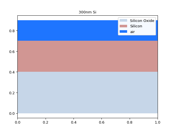
Using negative values for z_min will make the material stack grow. If you use a z_max value higher than the top of the material stack, it will grow as well.

mstack_c = mstack_b.clip_copy(z_min=-1, z_max=2.0)
mstack_c.visualize()