SMatrix1DSweep

class ipkiss3.all.circuit_sim.SMatrix1DSweep

A 3D matrix. The first two dimensions are related to the terms, the last dimension is related to a 1D sweep (i.e., wavelength sweep).

Parameters:

sweep_parameter_values: required

Values that are swept

sweep_parameter_name: str and String that contains only ISO/IEC 8859-1 (extended ASCII py3) or pure ASCII (py2) characters, required

Name of the parameter that is swept, e.g. ‘frequency’, ‘wavelength’

sweep_parameter_unit: ( str and String that contains only ISO/IEC 8859-1 (extended ASCII py3) or pure ASCII (py2) characters ), optional, *None allowed*

Unit of the sweep parameter, e.g. ‘GHz’, ‘um’. None = unknown.

terms: ( OrderedNamedTypedDict ), optional, *None allowed*

When term_modes is not given, we extract it from the the terms The term_modes pairs are added in consequetive blocks for each mode. The term_mode name is the following: - term_name, for the first mode with index 0: in - term_name_mode# for the modes with index higher than 0: in_1, in_2, in_3

term_modes: OrderedTypedDict, optional

Dictionary with { name (type: string)(term_name(type:string), mode (type: int/str)) } pairs: These are the (term-mode) pairs associated with the SMatrix. The dimension of the SMatrix equals len(term_modes) x len(term_modes). This dict is ordered: the order depends on the order they were added. This is useful if you want to ‘bulk’ set the S-matrix, S[:, :] = [[0, 1, 0], [0, 0, 1], [1, 0, 0]] : without the order information, setting these values is ambiguous.

symmetric: ( bool, bool_ or int ), optional

When True, the matrix is assumed to be symmetrical, and the associated component is a reciprocal component. This means the transmission from port x to y is equal to the transmission from port y to x.

n_ports: int and number > 0, optional

The number of simulated ports

term_mode_map: optional, *None allowed*

A dictionary that maps term,mode tuples to indices in the data array

dtype: type, optional

Type of the numpy array. By default, this is a complex number, because the scatter matrix contains both amplitude and phase information.

data: optional

Stores the raw data of the simulation results

static from_touchstone(filename, term_mode_map=None, unit=None)

Imports an S matrix frequency sweep from a touchstone file.

More information on the touchstone file format can be found in this document.

Parameters:

filename: str: filename to import
term_mode_map: dict: Maps (term, modenr) to TouchStone port_mode numbers. Use None for first attempting to derive from tool-specific parsing of the file header and when that fails assign default port names
unit: str: When specified, the sweep values will be converted to this unit. e.g. when the unit is ‘um’ the sweep_parameter_values will be in micrometer instead of the unit used in the touchstone file.

Returns:

smatrix: SMatrix1DSweep: 1D S matrix sweep

Examples

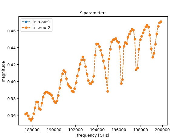
In this example we import a Touchstone file named ‘smatrix_fdtd.s6p’, made using the Link for Ansys Lumerical. You can download the Touchstone file and try the example below yourself. It represents a component with one input port and two output ports, where each port has 2 modes assigned to it. This configuration produces the number 6 (= 3 ports x 2 modes) in the extension. Also note how the file has a header containing metadata about the ports:

! Touchstone file export Luceda Link for Ansys Lumerical
! Luceda port in:mode 0:0
! Luceda port in:mode 1:1
! Luceda port out2:mode 0:2
! Luceda port out2:mode 1:3
! Luceda port out1:mode 0:4
! Luceda port out1:mode 1:5

This metadata is used by our importer if term_mode_map is set to None. It represents a mapping between ports in IPKISS/Lumerical and the Touchstone port numbers. For example, the second line maps the IPKISS port in:0 (= port in:mode 1) to Touchstone port 0.

import ipkiss3.all as i3
from ipkiss3.io.touchstone import import_touchstone_smatrix
import matplotlib.pyplot as plt
import numpy as np

S = import_touchstone_smatrix('smatrix_fdtd.s6p')

plt.figure()
plt.plot(S.sweep_parameter_values, np.abs(S["out1", "in"])**2, 'o--', label='in->out1', markersize=5)
plt.plot(S.sweep_parameter_values, np.abs(S["out2", "in"])**2, 'o--', label='in->out2', markersize=5)
plt.xlabel('frequency [GHz]')
plt.ylabel('magnitude')
plt.title('S-parameters')
plt.legend()
plt.show()

../../../../_images/ipkiss3-all-circuit_sim-SMatrix1DSweep-1.png

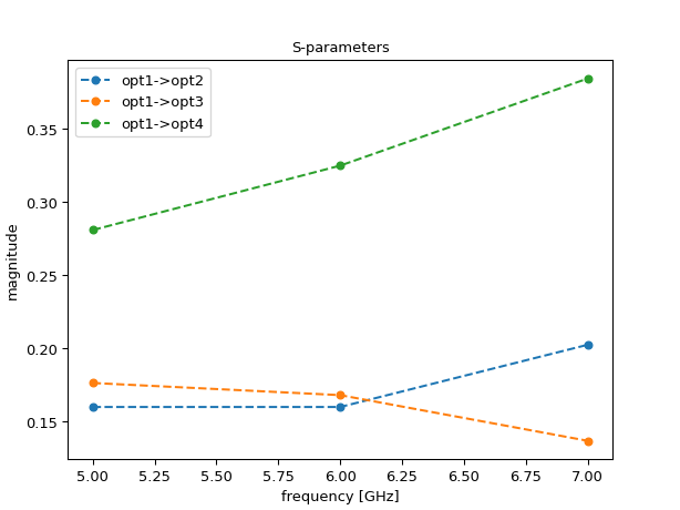
The next example shows how to set your own term_mode_map:

import ipkiss3.all as i3
from ipkiss3.io.touchstone import import_touchstone_smatrix
import matplotlib.pyplot as plt
import numpy as np
touchstone_4port = '''! 4-port S-parameter data, taken at three frequency points
# GHZ S MA R 50
5.00000 0.60 161.24 0.40 -42.20 0.42 -66.58 0.53 -79.34 !row 1
        0.40 -42.20 0.60 161.20 0.53 -79.34 0.42 -66.58 !row 2
        0.42 -66.58 0.53 -79.34 0.60 161.24 0.40 -42.20 !row 3
        0.53 -79.34 0.42 -66.58 0.40 -42.20 0.60 161.24 !row 4
6.00000 0.57 150.37 0.40 -44.34 0.41 -81.24 0.57 -95.77 !row 1
        0.40 -44.34 0.57 150.37 0.57 -95.77 0.41 -81.24 !row 2
        0.41 -81.24 0.57 -95.77 0.57 150.37 0.40 -44.34 !row 3
        0.57 -95.77 0.41 -81.24 0.40 -44.34 0.57 150.37 !row 4
7.00000 0.50 136.69 0.45 -46.41 0.37 -99.09 0.62 -114.19 !row 1
        0.45 -46.41 0.50 136.69 0.62 -114.19 0.37 -99.09 !row 2
        0.37 -99.09 0.62 -114.19 0.50 136.69 0.45 -46.41 !row 3
        0.62 -114.19 0.37 -99.09 0.45 -46.41 0.50 136.69 !row 4
'''
filename = "touchstone_4port_example.s4p"

with open(filename, 'w') as f:
    f.write(touchstone_4port)

term_mode_map = {
    ("opt1", 0): 0,
    ("opt2", 0): 1,
    ("opt3", 0): 2,
    ("opt4", 0): 3
}

S = import_touchstone_smatrix(filename, term_mode_map=term_mode_map)

plt.figure()
plt.plot(S.sweep_parameter_values, np.abs(S["opt2", "opt1"])**2, 'o--', label='opt1->opt2', markersize=5)
plt.plot(S.sweep_parameter_values, np.abs(S["opt3", "opt1"])**2, 'o--', label='opt1->opt3', markersize=5)
plt.plot(S.sweep_parameter_values, np.abs(S["opt4", "opt1"])**2, 'o--', label='opt1->opt4', markersize=5)
plt.xlabel('frequency [GHz]')
plt.ylabel('magnitude')
plt.title('S-parameters')
plt.legend()
plt.show()

../../../../_images/ipkiss3-all-circuit_sim-SMatrix1DSweep-2.png

to_touchstone(filename, reference=50.0, param_format='MA')

Exports an S matrix frequency / wavelength sweep to a touchstone file.

More information on the touchstone file format can be found in this document.

Parameters:

smatrix1dsweep: SMatrix1DSweep: stores the SMatrices from a sweep
filename: str: filename to which to export. The standard TouchStone extension .snp with n the total number of port modes will automatically be appended if not specified by the user. (e.g. s6p if there are 3 ports and each has 2 modes)
reference: float (default 50.): Reference in ohms. Used as a system reference for the S matrix data.
param_format: str: Format of the output MA: magnitude and angle (in degrees) in the counter-clockwise directions RI: real and imaginary part
n_digits: int (default 17): Number of significant digits in the output Touchstone file. The default value is chosen such that when IEEE 754 double-precision number is converted to a decimal string and back the original and converted value must match (see https://en.wikipedia.org/wiki/Double-precision_floating-point_format)

Returns:

filename: str: The exported full file path including extension

passivity_check()

Check if the SMatrix1DSweep is passive.

Parameters:

smatrix1dsweep: SMatrix1DSweep: stores the SMatrices from a sweep

Returns:

indices: A numpy array that contains the indices of the sweep values that: are not passive

Examples

>>> smat = i3.device_sim.SMatrix1DSweep.from_touchstone('mydc.s4p')
>>> indices = smat.passivity_check()
>>> non_passivity_wls = smat.sweep_parameter_values[indices]
>>> is_passive = len(indices) == 0

reciprocity_check()

Check if the SMatrix1DSweep is reciprocal.

Parameters:

smatrix1dsweep: SMatrix1DSweep: stores the SMatrices from a sweep

Returns:

indices: A numpy array that contains the indices of the sweep values that: are not reciprocal

Examples

>>> smat = i3.device_sim.SMatrix1DSweep.from_touchstone('mydc.s4p')
>>> indices = smat.reciprocity_check()
>>> non_reciprocal_wls = smat.sweep_parameter_values[indices]
>>> is_reciprocal = len(indices) == 0

visualize(terms=None, term_pairs=None, figsize=(8, 8), scale='linear', show=True, title=None, xlabel=None, ylabel=None, legend=True, xrange=None, yrange=None, figure=None, save_name=None, dB_min=-120)

Visualize the S-matrix sweep.

Parameters:

terms: Optional[List[str]]: List of terms for which to plot the S-parameters. Plots every combination between these given terms. If specified together with term_pairs, an error will be raised. If None, will plot the pairs of terms according to the term_pairs argument. If term_pairs is also None, will plot every combination between all available terms.
term_pairs: Optional[List[Tuple[str, str]]]: List of term pairs for which to plot the S-parameters. The order in the tuple is (“in”, “out”), i.e. to retrieve the transmission from “in” to “out” defined by s_matrix[“out”, “in”], term_pairs should be [(“in”, “out”)]. If specified together with terms, an error will be raised. If None, will plot the combinations according to the terms argument. If terms is also None, will plot every combination between all available terms.
figsize: Tuple[float, float]: Size of the figure (width, height) in inches. Default is (8, 8)
scale: Literal[‘linear’, ‘dB’]: Scale of the wavelength/frequency. ‘linear’ or ‘dB’. Default is ‘linear’.
show: bool: If True, the plot will be shown. Default is True.
title: Optional[str]: Title of the plot. If None, no title will be displayed.
xlabel: Optional[str]: The label of the x-axis. If None, it will be set automatically based on the sweep parameter unit.
ylabel: Optional[str]: The label of the y-axis. If None, the axis will be labelled S-parameters [abs. units] if scale is linear or S-parameters [dB] if scale is dB.
legend: bool: If True, the legend will be shown. Default is True.
xrange: Optional[Tuple[float, float]]: The range of x-axis to be plotted.
yrange: Optional[Tuple[float, float]]: The range of y-axis to be plotted.
figure: Optional[Figure]: Matplotlib Figure to plot on. If None, a new figure is generated.
save_name: Optional[str]: If provided, the figure will be saved with the given name. For headless mode, show still need to be put on False.
dB_min: float: The minimum threshold for dB values. Any values lower than this threshold will be rounded up to this specified minimum value. This parameter is applicable only when the scale is set to ‘dB’. Default is -120.

Returns:

None or matplotlib.figure.Figure: None if running from a jupyter notebook or if show is true, the Matplotlib Figure object otherwise

visualize_map(figsize=(8, 8), scale='linear', sweep_value=None, show=True, title=None, ylabel=None, figure=None, save_name=None, dB_min=-120)

Plot S-parameters as a map.

Parameters:

figsize: Tuple[float, float]: Size of the figure, default is (8, 8).
scale: Literal[‘linear’, ‘dB’]: Scale of the wavelength/frequency, choose between ‘linear’ or ‘dB’. Default is ‘linear’.
sweep_value: Optional[float]: Evaluated wavelength or frequency. If None, the middle is chosen. If the value is not in the data, the closest value is chosen instead.
show: bool: If True, the plot will be displayed. Default is True.
title: Optional[str]: Title of the plot. If None, no title will be displayed.
ylabel: Optional[str]: The label of the y-axis. If None, the axis will be labelled S-parameters [abs. units] if scale is linear or S-parameters [dB] if scale is dB.
figure: Optional[Figure]: Matplotlib Figure to plot on. If None, a new figure is generated.
save_name: Optional[str]: If provided, the figure will be saved with the given name.
dB_min: Optional[float]: The minimum threshold for dB values. Any values lower than this threshold will be rounded up to this specified minimum value. This parameter is applicable only when the scale is set to ‘dB’. Default is -120.

Returns:

None or matplotlib.figure.Figure: None if running from a jupyter notebook or if show is true, the Matplotlib Figure object otherwise