Tidy3D

When you set up an electromagnetic simulation using Tidy3D from within IPKISS, you go through the following steps:

Define the geometry that represents your component.
Specify the simulation job, consisting of the geometry, the expected outputs and simulation settings.
Inspect the exported geometry.
Retrieve the simulation results.

Note

Tidy3D comes bundled within our installer, but before using Tidy3D you will need to create a Tidy3D account and set up your API key inside your environment. Once you have obtained your API key, either setup the SIMCLOUD_APIKEY environment variable or open the ipkiss terminal from Luceda Control Center to register the key.

# Windows
C:\luceda\luceda_2024090\envs\device_sim\Scripts\tidy3d.exe configure --apikey=XXX
# Linux
~/miniconda/envs/device_sim/bin/tidy3d configure --apikey=XXX

For a more detailed guide on how to set up Tidy3D, you can follow their documentation (you can skip the pip install step): https://docs.flexcompute.com/projects/tidy3d/en/latest/install.html#getting-started.

1. Define the geometry

We’ve already covered step 1 in the following guide: creating a SimulationGeometry for an MMI. However we will adjust the geometry a bit by growing the waveguides slightly (this happens also automatically, if waveguide_growth is not specified waveguide_growth=1.1*center_wavelength). This is important to ensure the structure sufficiently extends beyond the edge of the simulation window (bounding_box), in the case where perfectly matched layers (PMLs) are applied. PMLs are the default boundary conditions. If not specified, the simulation bounding box will be automatically based on the simulation geometry before growing waveguides, with a margin added in x and y directions to make sure all ports are sufficiently enclosed in the simulation window.

sim_geom = i3.device_sim.SimulationGeometry(
    layout=MMI_lo,
    waveguide_growth=2.0,
)

This makes sure the ports don’t fall at the edge of the simulation region, and the waveguides extend into the PML so that any field going out of the device is absorbed. The next step is to create an object that will handle the simulations.

2. Define the simulation

To create a simulation using the geometry we’ve just defined, we will instantiate a i3.device_sim.Tidy3DFDTDSimulation object:

simulation = i3.device_sim.Tidy3DFDTDSimulation(
  geometry=sim_geom,
  monitors=[
    i3.device_sim.Port(name="in1", box_size=(2.0, 1.0)),
    i3.device_sim.Port(name="out1", box_size=(2.0, 1.0)),
    i3.device_sim.Port(name="out2", box_size=(2.0, 1.0)),
  ],
  center_wavelength=1.55,
  outputs=[i3.device_sim.SMatrixOutput(name="smatrix", wavelength_range=(1.5, 1.6, 50))],
  setup_macros=[
      i3.device_sim.tidy3d_macros.fdtd_auto_grid_spec(min_steps_per_wavelength=15),
      i3.device_sim.tidy3d_macros.fdtd_profile_xy(alignment_port="in1"),
  ],
  task_name="soi_mmi_fdtd",
  task_folder_name="mmi_simulation",
)

This sets up our simulation object, with the correct geometry, ports and expected results. It sets the center_wavelength at which the simulation will be performed. The monitors are overridden to avoid overlap (see Monitors). When specifying SMatrixOutput, the simulator will perform an S-parameter sweep and return an SMatrix (i3.circuit_sim.Smatrix1DSweep). In this case, monitors will act both as Tidy3D sources and monitors (and will be passed to the Tidy3D ComponentModeler class.) Tidy3D will perform separate simulations, exciting each port. The MMI has three ports, i.e. three simulations will be performed. For an S-parameter sweep, Tidy3D’s ComponentModeler runs the simulations with a modal source.

We have also added two macros:

fdtd_auto_grid_spec allows to control the number of points per center_wavelength in the mesh of the component in Tidy3D FDTD.
fdtd_profile_xy lets us place an XY field monitor (with its Z position aligned to a specified port) and visualize the results (like the electric field) after the simulation is done.

In addition, there are a few parameters that allow you to customize where to store the simulations:

task_name specifies the name of the task when setting up the simulation. This would be the name under which the geometry setup will be saved in the Tidy3D web interface.
task_folder_name specifies the name of the Tidy3D folder to which the geometry and the results are saved. Default is the cell name.
project_folder allows you to choose where to save the simulation data, scripts, and outputs locally. In addition to this, all simulation outputs will be downloaded to the data folder, under the project_folder. Default is the current working directory.

Now everything is set up to start Tidy3D and do our first simulation.

3. Inspect the simulation job

To see what it looks like, you can use the inspect method:

simulation.inspect()

After execution, a web interface of Tidy3D and a matplotlib figure will open:

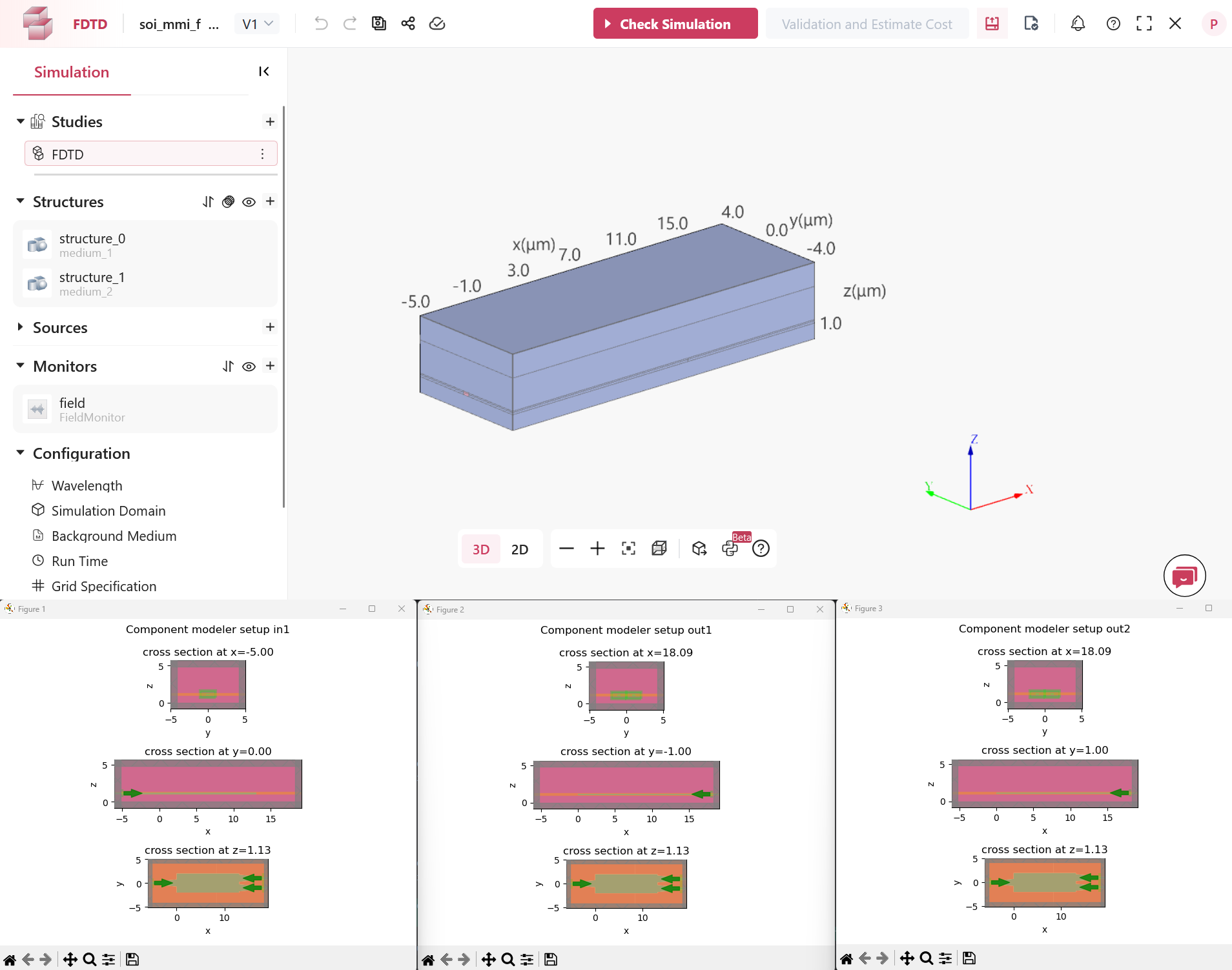
The web interface of Tidy3D allows you to explore the Simulation setup. You can now inspect the geometry, materials (extracted from the PDK definitions where possible), estimate the simulation cost, and other settings as exported by IPKISS. You can make changes and modify settings from here. See macros below on how to make those settings available for future projects. The web interface contains no information about the whereabouts of the ports.

In addition, figure pop-ups (one for each port) show the setup of the ComponentModeler, which is used to compute the scattering matrix (for more details see the documentation of Tidy3D). This allows to inspect the geometry and the location, size and direction of the mode ports.

4. Retrieve and plot simulation results

After you’ve confirmed that the simulation setup is correct, you can run the simulation and retrieve the results from the outputs. By default you don’t have to launch the simulation explicitly; when you request the results, IPKISS will run the simulation when required.

smatrix = simulation.get_result(name='smatrix')

Note

By default, the S-matrix that is returned after the simulation will have its sweep units in micrometer. This is in contrast to manually importing the S-matrix touchstone file using import_touchstone_smatrix, in which case the default sweep units are in GHz.

You can now plot these S-parameters with smatrix.visualize() (visualize). or they can be stored to disk (S-parameter data handling). Our link will also create a touchstone file named ‘smatrix.s3p’ that can be imported using import_touchstone_smatrix.

smatrix.visualize(
    scale="dB",
    term_pairs=[
        ("in1", "out1"),
        ("out1", "out2"),
        ("in1", "in1"),
    ],
    yrange=[-60, 0.1],
)

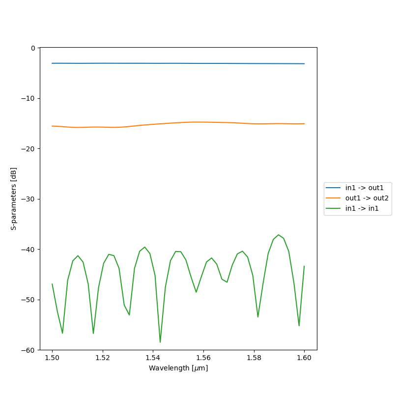
Only the transmission to the ‘out1’ port is plotted because the MMI is symmetric. We see that around half of the power is transmitted to each output port, but the MMI can be optimized further.

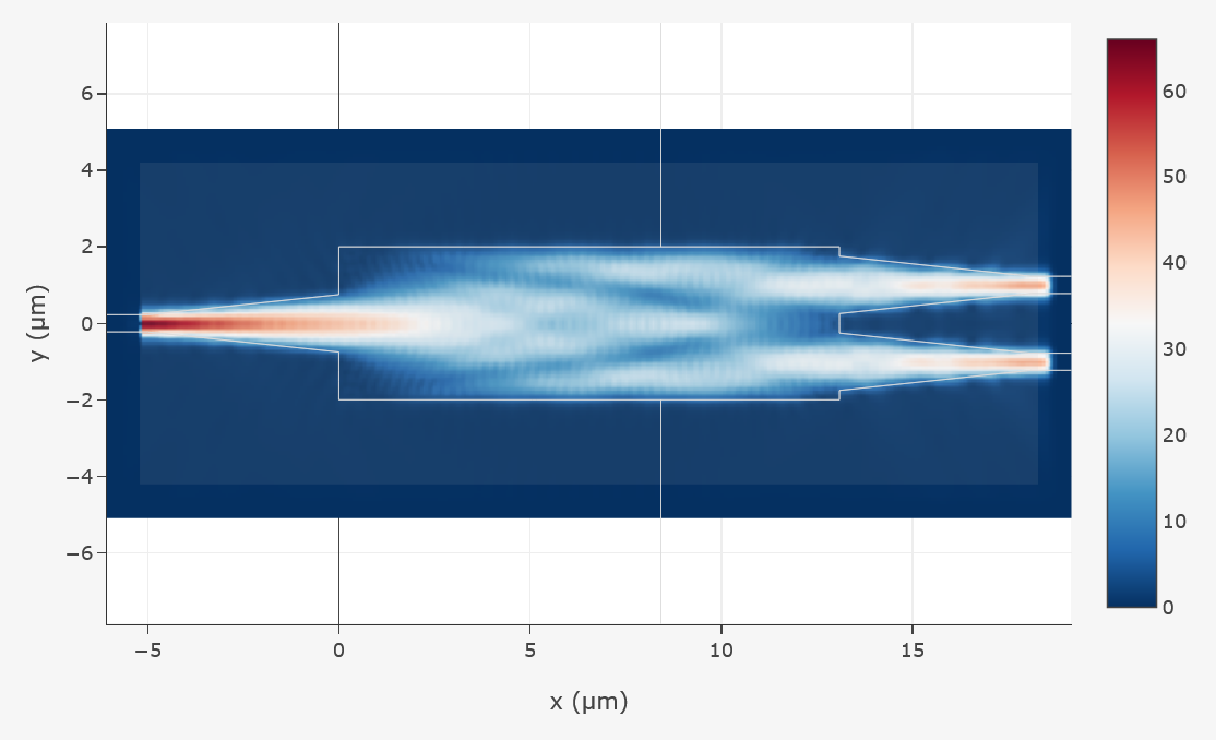
The distribution of electric field (with the input port excited in the figure below) can be visualized thanks to the monitor we placed earlier:

Note

When called, both simulation.inspect and simulation.get_result will output a simulation.py to the project_folder, which is the script that we run programmatically. It can also be tweaked for desired behavior by writing Tidy3D specific code, and running it manually.

5. Advanced simulation settings

Monitors

Just as is the case with the geometry, IPKISS sets reasonable defaults for the port monitors. When you don’t specify any ports, defaults will automatically be added. The default position, direction are directly taken from the OpticalPorts of the layout, the dimensions of the Ports are calculated with a heuristic. Specifically, the width of the port is taken from the core_width attribute of the trace_template of the IPKISS OpticalPort. Any waveguide template that is a WindowWaveguideTemplate will have this attribute. For the majority of waveguide templates this is the case. The heuristic will add a fixed margin of 1 um to this core_width. The height of the port is derived from the Material Stack used to virtually fabricate the layer of the core of the Waveguide, searching for the highest refractive index region but excluding the bottom, top, left and right boundary materials.

Still, if the inputs/outputs are close together (<1 um), then the monitors will overlap and double count the e-field, which is also something that Tidy3D reports. This is why the monitor defaults were overridden by using the monitors argument in the simulation class of the main example. The example code below illustrates how to use monitors of different sizes.

simulation = i3.device_sim.Tidy3DFDTDSimulation(
    geometry=sim_geom,
    monitors=[
        # override the ports so that their center and size is reproducible
        i3.device_sim.Port(
            name="in1",
            box_size=(5.0, 2.0),
        ),
        i3.device_sim.Port(
            name="out1",
            box_size=(2.0, 1.0),
        ),
        i3.device_sim.Port(
            name="out2",
            box_size=(2.0, 1.0),
        ),
    ],
    outputs=[i3.device_sim.SMatrixOutput(name="smatrix", wavelength_range=(1.5, 1.6, 50))],
)

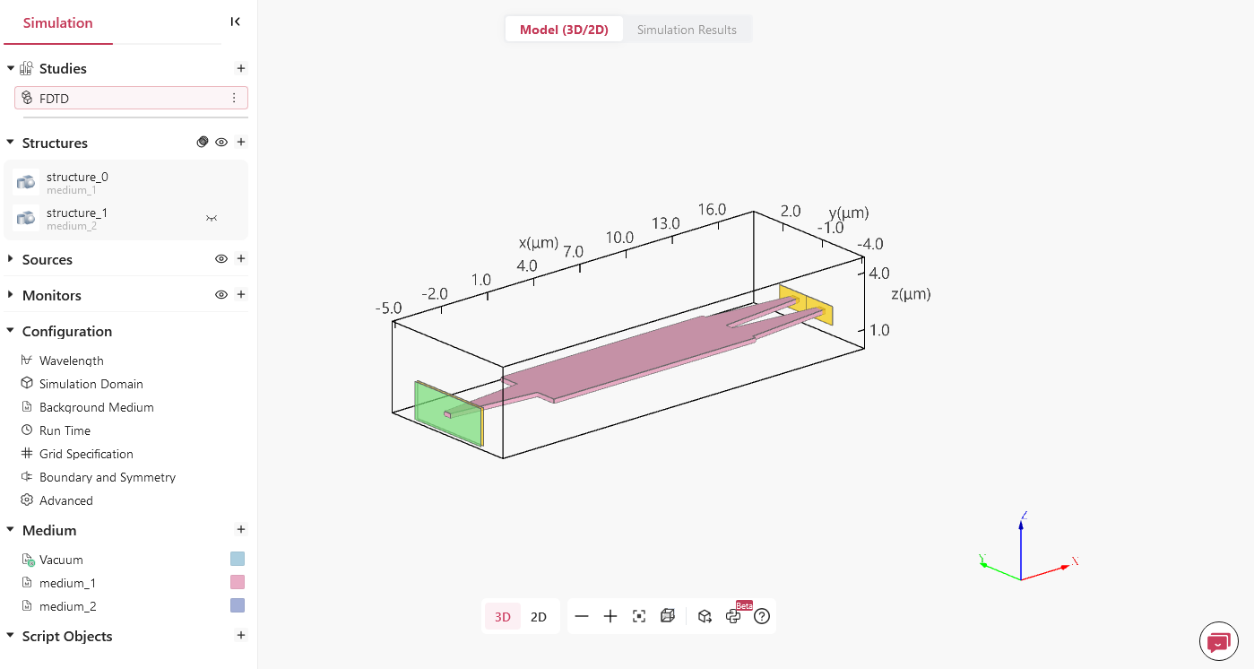
When you inspect the simulation object for a certain scattering matrix source (accessible through the main Tidy3D workspace) you’ll see something similar to the picture below:

Multimode waveguides

By default, waveguide ports will be simulated with a single mode (the fundamental mode). You can override this in order to take multiple modes into account (note that this doesn’t allow controlling the polarisation):

simulation = i3.device_sim.Tidy3DFDTDSimulation(
   geometry=sim_geom,
   monitors=[i3.device_sim.Port(name="in1", box_size=(2.0, 1.0), n_modes=2),
             i3.device_sim.Port(name="out1", box_size=(2.0, 1.0), n_modes=2),
             i3.device_sim.Port(name="out2", box_size=(2.0, 1.0), n_modes=2)],
   outputs=[
      i3.device_sim.SMatrixOutput(
         name='smatrix',
         wavelength_range=(1.5, 1.6, 100),
         symmetries=[('out1', 'out2')]
      )
   ]
)

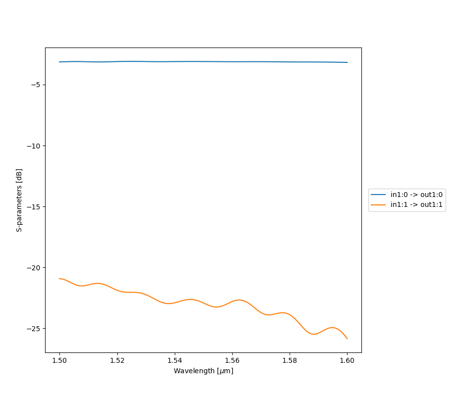
The simulation results will then contain the S-parameters for each port-mode combination:

smatrix = simulation.get_result(name="smatrix")
smatrix.visualize(
  scale="dB",
  term_pairs=[
      ("in1:0", "out1:0"),
      ("in1:1", "out1:1"),
  ],
)

6. Tool-specific settings

In addition to the generic settings that can be applied to multiple solvers, the IPKISS device simulation interface also allows users to use the full power of the solver tool. Tool-specific materials can be used and tool-specific macros can be defined.

Using materials defined by the simulation tool

By default, IPKISS exports materials for each material used in the process flow definition.

You can also reuse materials which are already defined by the device solvers by specifying a dictionary solver_material_map to the simulation object (Tidy3DFDTDSimulation). It maps IPKISS materials onto materials defined by the tool (name-based).

For example:

simulation = i3.device_sim.Tidy3DFDTDSimulation(
    ....
    solver_material_map={
        TECH.MATERIALS.SILICON: "cSi - Palik_Lossless",
        TECH.MATERIALS.SILICON_OXIDE: "SiO2 - Palik_Lossless",
    },
)

This will map the TECH.MATERIALS.SILICON, and SILICON_OXIDE, onto materials defined by the electromagnetic solver. The material name should be know by the solver. Please check the tool documentation to find out which materials are available.

Macros

Setting `tidy3d.Simulation` parameters

Often you will want to tweak certain settings (simulation settings, materials, …) using very tool-specific commands or actions. When inspecting the simulation project from the Tidy3D web interface, one can easily tweak any desired settings. The same is possible by using the Python API of Tidy3D.

Since it is not feasible to abstract everything, IPKISS provides a way to apply tool-specific settings using macros. They allow you to add tool-specific commands using their API. We have already demonstrated this above by customizing the mesh in Tidy3D FDTD. The setup_macros argument allows to set specific parameters of tidy3d.Simulation.

IPKISS provides some premade macros which are available under the i3.device_sim.tidy3d_macros namespace, and you can visit the documentation for more information.

As an example how to write a Macro, here we specify the run_time variable, which allows you to control the runtime of your simulation:

macro = i3.device_sim.Macro(commands=["run_time = 1e-12"])
simulation = i3.device_sim.Tidy3DFDTDSimulation(
    geometry=sim_geom,
    setup_macros=[macro],
    outputs=[i3.device_sim.SMatrixOutput(name="smatrix", wavelength_range=(1.5, 1.6, 50))],
)

Note that we expose all variables that the tidy3d.Simulation class can accept under the same name (other examples are monitors, symmetry, …). size and center variables are controlled via the bounding_box and are not exposed.

Generating output files

You can also use macros to execute tool-specific code to generate output files and retrieve those with simulation.get_result. In the following example we use it to generate a file with value of the effective index .

simulation = i3.device_sim.Tidy3DFDTDSimulation(
    geometry=sim_geom,
    outputs=[
        i3.device_sim.MacroOutput(
            name="macro-output",
            # filepath must correspond with the file used in the commands.
            filepath="numbers.txt",
            commands=[
                "a=range(5)",
                'with open("numbers.txt", "w+") as output_file:',
                "    for idx in a:",
                '        output_file.write(str(idx) + " ")',
        ],
        )
    ],
)

# get_result will execute the code and take care of copying the file when required.
fpath = simulation.get_result('macro-output')
print(open(fpath).read())
# expected output:
# 0 1 2 3 4

7. Building models based on simulation results

Finally, when you are satisfied with the S-matrix you obtained, you can store it in the Touchstone format. Then, you can use it to build a CircuitModel for your PCell, see Physical device simulation guide and Circuit simulation with scatter matrix files.

Tidy3D

1. Define the geometry

2. Define the simulation

3. Inspect the simulation job

4. Retrieve and plot simulation results

5. Advanced simulation settings

Monitors

Multimode waveguides

6. Tool-specific settings

Using materials defined by the simulation tool

Macros

Setting tidy3d.Simulation parameters

Generating output files

7. Building models based on simulation results

Setting `tidy3d.Simulation` parameters